These are the notes I put together while learning optimal transport (OT). They mainly follow Peyré & Cuturi’s Computational Optimal Transport and Cuturi’s 2013 Sinkhorn paper, which is also where most of the figures come from.
1. The problem in brief
Given a source distribution and a target distribution, we want to “move” the source onto the target at the lowest total cost. Here \(c(m,n)\) is the cost of moving one unit of mass from \(m\) to \(n\), and what we solve for is the optimal transport plan \(p(m,n)\).
Once we have the minimal total cost and the optimal plan, we can:
- use the minimal total cost to measure how similar or different the two distributions are;
- under suitable conditions, use the plan \(p(m,n)\) to transfer new samples in the same way.
2. Basic concepts
2.1 Definitions
Histograms (probability vectors): an array of length \(n\) whose entries lie in \([0, 1]\) and sum to 1, i.e. a discrete probability distribution:
\[\Sigma_n \overset{\text{def.}}{=} \left\{ \mathbf{a} \in \mathbb{R}_{+}^n : \sum_{i=1}^n \mathbf{a}_i = 1 \right\}\]Discrete measures: a discrete measure with weights \(\mathbf{a}\) and locations \(x_1, \ldots, x_n \in \mathcal{X}\) is written
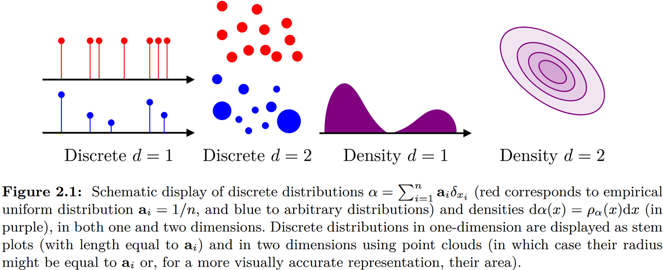
\[\alpha=\sum_{i=1}^n \mathbf{a}_i \delta_{x_i}\]In the figure below, red dots are uniform distributions (\(\mathbf{a}_i = 1/n\)) and blue dots are arbitrary ones. In 1-D, a discrete distribution is drawn as stems (length = weight); in 2-D, as a point cloud (dot size = weight).
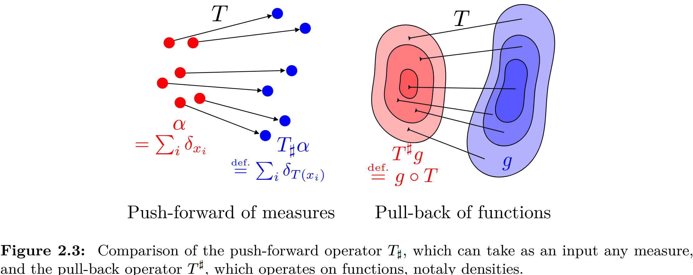
Push-forward operator: for a continuous map \(T:\mathcal{X}\to\mathcal{Y}\), the push-forward operator is \(T_\sharp:\mathcal{M}(\mathcal{X})\to\mathcal{M}(\mathcal{Y})\). For a discrete measure, it simply moves every point to its image under \(T\):
\[T_\sharp\alpha\overset{\text{def.}}{=}\sum_i\mathbf{a}_i\delta_{T(x_i)}\]Intuitively, a measurable map \(T\) moves a point in one space to a point in another, and \(T_\sharp\) extends this from single points to whole probability measures: it “pushes” one measure forward into a new one.
2.2 The Monge problem
2.2.1 Definition
The Monge problem: find a map from one measure to another that minimizes the sum of all \(c(x_i, T(x_i))\), where \(c\) is the transport cost and has to be defined for the application at hand.
In the discrete setting, given two discrete measures
\[\alpha=\sum_{i=1}^n \mathbf{a}_i \delta_{x_i} \quad \text{and} \quad \beta=\sum_{j=1}^m \mathbf{b}_j \delta_{y_j}\]we look for a map \(T:\{x_1,\ldots,x_n\}\to\{y_1,\ldots,y_m\}\) such that
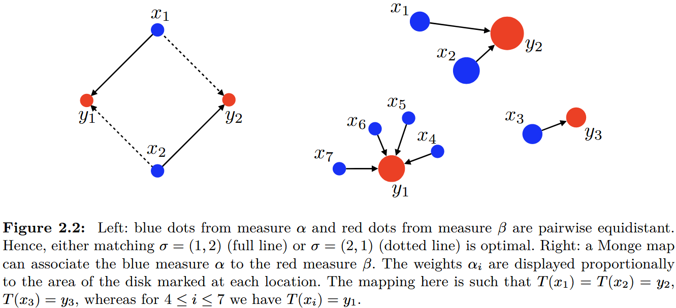
\[\forall j \in [\![ m ]\!], \quad \mathbf{b}_j=\sum_{i: T(x_i)=y_j} \mathbf{a}_i\]This constraint can be written compactly as \(T_{\sharp} \alpha=\beta\) and is called the mass conservation constraint.
- When \(n=m\) and the weights are uniform, \(T\) is a one-to-one matching (left figure below);
- When \(n>m\), each \(x_i\) must be sent as a whole to a single \(y_j\), but a \(y_j\) can receive several \(x_i\) (right figure);
- When \(n<m\) (and all \(\mathbf{b}_j > 0\)), at most \(n\) of the \(y_j\) can receive any mass, so the constraint cannot be met and the problem has no solution.
Putting it together, the problem is
\[\min_T\left\{\sum_i c\left(x_i, T\left(x_i\right)\right): T_{\sharp} \alpha=\beta\right\}\]In words: through the map \(T\), every \(\mathbf{a}_i\) must be shipped, and each \(\mathbf{b}_j\) must receive exactly its own amount. \(c\) is the transport cost and \(T\) is the transport plan.
2.2.2 Limitations
- A feasible solution may not exist: e.g. the \(n<m\) case above.
- The feasible set is non-convex and hard to optimize: the push-forward in the mass conservation constraint is combinatorial, so optimization is hard and often comes down to enumerating plans, which is extremely expensive.
So can we drop the requirement that transport be a deterministic map, and turn OT into a convex problem? Then:
- a feasible solution always exists (e.g. \(\mathbf{a}\mathbf{b}^{\mathrm{T}}\));
- we can use a wide range of optimization methods to solve it.
This is the Kantorovich relaxation.
2.3 The Kantorovich relaxation
2.3.1 The transport polytope
Kantorovich’s key idea is to relax the deterministic nature of transport. In the Monge problem, a source point \(x_i\) must be assigned as a whole to a single location \(T(x_i)\); Kantorovich instead allows the mass at \(x_i\) to be split and sent to several targets. In other words, deterministic transport is replaced by probabilistic transport.
For probability vectors \(\mathbf{a}\in\Sigma_n\) and \(\mathbf{b}\in\Sigma_m\), the set of admissible transport plans (couplings) is
\[\mathbf{U}(\mathbf{a}, \mathbf{b}) \stackrel{\text{def.}}{=}\left\{\mathbf{P} \in \mathbb{R}_{+}^{n \times m}: \mathbf{P} \mathbf{1}_m=\mathbf{a} \quad \text{and} \quad \mathbf{P}^{\mathrm{T}} \mathbf{1}_n=\mathbf{b}\right\}\]where
\[\mathbf{P} \mathbf{1}_m=\Big(\sum_j \mathbf{P}_{i, j}\Big)_i \in \mathbb{R}^n \quad \text{and} \quad \mathbf{P}^{\mathrm{T}} \mathbf{1}_n=\Big(\sum_i \mathbf{P}_{i, j}\Big)_j \in \mathbb{R}^m\]That is, the rows of \(\mathbf{P}\) sum to \(\mathbf{a}\) and its columns sum to \(\mathbf{b}\). The right side of the figure below draws a discrete coupling as a matrix, with disk size proportional to \(\mathbf{P}_{i,j}\):
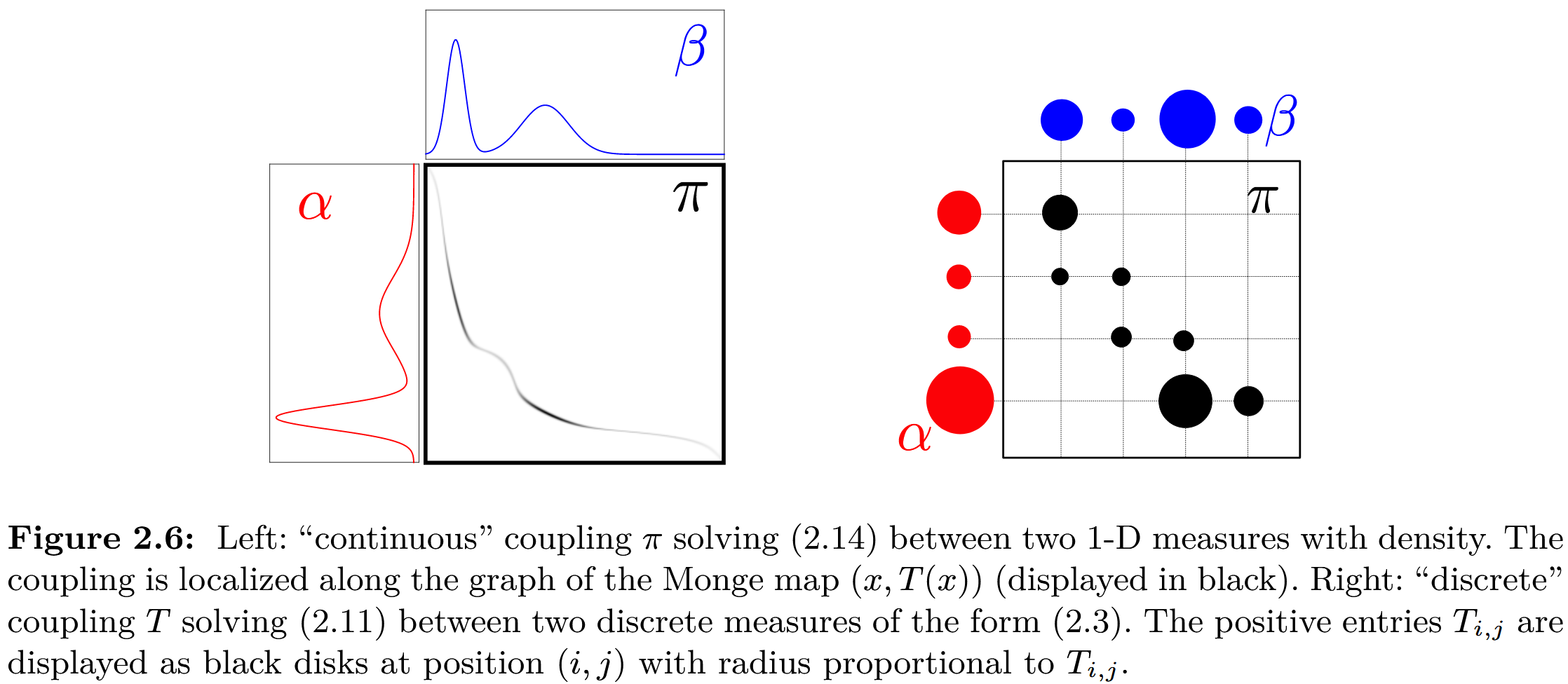
\(\mathbf{U}(\mathbf{a},\mathbf{b})\) is defined by \(n+m\) linear equality constraints plus non-negativity, so it is a bounded convex polytope (the convex hull of finitely many matrices).
Also, the Monge problem is inherently asymmetric (see the right Monge example above: \(x_4,\ldots,x_7\) can merge into \(y_1\), but \(y_1\) cannot be split back into them), whereas the Kantorovich relaxation is always symmetric: \(\mathbf{P}\in\mathbf{U}(\mathbf{a},\mathbf{b})\) if and only if \(\mathbf{P}^{\mathrm{T}}\in\mathbf{U}(\mathbf{b},\mathbf{a})\).
2.3.2 The objective and how to read it
The resulting optimization problem is
\[\mathrm{L}_{\mathbf{C}}(\mathbf{a}, \mathbf{b}) \stackrel{\text{def.}}{=} \min_{\mathbf{P} \in \mathbf{U}(\mathbf{a}, \mathbf{b})}\langle\mathbf{C}, \mathbf{P}\rangle \stackrel{\text{def.}}{=} \sum_{i, j} \mathbf{C}_{i, j} \mathbf{P}_{i, j}\]Some ways to read it:
- The inner product of \(\mathbf{C}\) and \(\mathbf{P}\) should be as small as possible, i.e. pairs of points with lower transport cost get larger matching weights \(\mathbf{P}_{i,j}\);
- Kantorovich relaxes the constraint, allowing many-to-many matching between \(x\) and \(y\);
- The rows of \(\mathbf{P}^*\) sum to \(\mathbf{a}\) and its columns to \(\mathbf{b}\), i.e. total input and output must match;
- Since the row and column sums of \(\mathbf{P}^*\) are both probability distributions, \(\mathbf{P}^*\) can also be read as a joint probability distribution.
2.3.3 Monge vs. Kantorovich
- Motivation: Kantorovich relaxes Monge’s mass conservation constraint by introducing mass splitting: the mass at a source point \(x_i\) can be spread across different destinations;
- Idea: from deterministic transport to probabilistic transport;
- Solving: the Monge problem is non-convex and may have no feasible solution; the Kantorovich problem is a linear program, always has an optimal solution, and can be solved with mature LP methods;
- Generality: the Kantorovich formulation greatly broadens where OT can be applied.
3. Algorithms
3.1 Exact solutions
Solving OT usually means solving the Kantorovich relaxation, which is a linear program.
3.1.1 Vertices of the transport polytope
A linear program with a non-empty, bounded feasible set always attains its minimum at some vertex of that set. Since \(\mathbf{U}(\mathbf{a},\mathbf{b})\) is bounded, the search for an optimal \(\mathbf{P}\) can be restricted to the vertices (extreme points) of \(\mathbf{U}(\mathbf{a},\mathbf{b})\).
3.1.2 A bipartite-graph view
OT can be viewed as a network flow problem on a bipartite graph: \(n\) source nodes on the left, \(m\) target nodes on the right, each edge \((i, j')\) has cost \(\mathbf{C}_{i,j}\), and \(\mathbf{P}_{i,j}\) is the flow on that edge.
A key result: \(\mathbf{P}\) is a vertex of \(\mathbf{U}(\mathbf{a},\mathbf{b})\) if and only if its edges with non-zero flow contain no cycle. This also means a vertex solution has at most \(n+m-1\) non-zero flows.
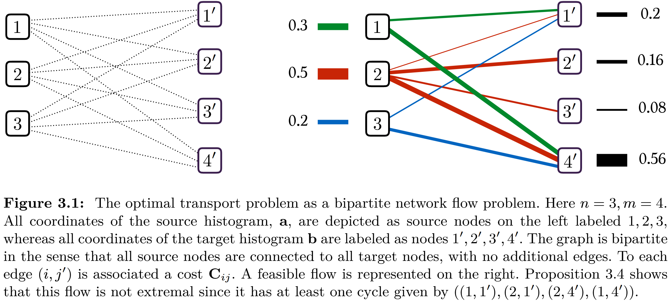
Each line on the right is a flow of mass. It contains the cycle \((1,1'),(2,1'),(2,4'),(1,4')\), so it is not a vertex. This is the geometric picture behind solving OT.
3.1.3 North-west corner rule and network simplex
- North-west corner rule: start from the top-left entry of the matrix. At each step, put the smaller of “what is left of \(\mathbf{a}_i\)” and “what is left of \(\mathbf{b}_j\)” into the current cell, then move down or right depending on which one ran out. After at most \(n+m-1\) steps this gives a vertex solution: feasible, but usually not optimal.
- Network simplex: start from the north-west corner solution. At each step, add an edge that lowers the total cost and shift flow along the cycle it creates, moving between adjacent vertices until no better neighbor exists.
For \(n\) points, exact solvers cost roughly \(O(n^3\log n)\), which gets slow quickly as the data grows. This is the motivation for entropic regularization.
3.2 Entropic regularization
In most applications, the exact solution of the Kantorovich problem is not needed: solving a regularized version approximately makes OT far cheaper. The entropy is defined as
\[\mathbf{H}(\mathbf{P}) \stackrel{\text{def.}}{=}-\sum_{i, j} \mathbf{P}_{i, j}\left(\log \mathbf{P}_{i, j}-1\right)\]\(\mathbf{H}\) is 1-strongly concave, since \(\partial^2 \mathbf{H}(\mathbf{P})=-\operatorname{diag}\left(1 / \mathbf{P}_{i, j}\right)\) and \(\mathbf{P}_{i, j} \leq 1\). Entropic regularization uses \(-\mathbf{H}\) as the regularizer and solves for an approximate solution:
\[\mathrm{L}_{\mathbf{C}}^{\varepsilon}(\mathbf{a},\mathbf{b}) \stackrel{\text{def.}}{=} \min_{\mathbf{P} \in \mathbf{U}(\mathbf{a},\mathbf{b})}\langle \mathbf{P},\mathbf{C}\rangle - \varepsilon \mathbf{H}(\mathbf{P})\]The figure below shows the effect of \(\varepsilon\): at \(\varepsilon = 0\) the solution sits on a vertex of the feasible set (the LP solution); as \(\varepsilon\) grows, the entropy pushes the solution away from the boundary toward the “entropic center” inside the feasible set.
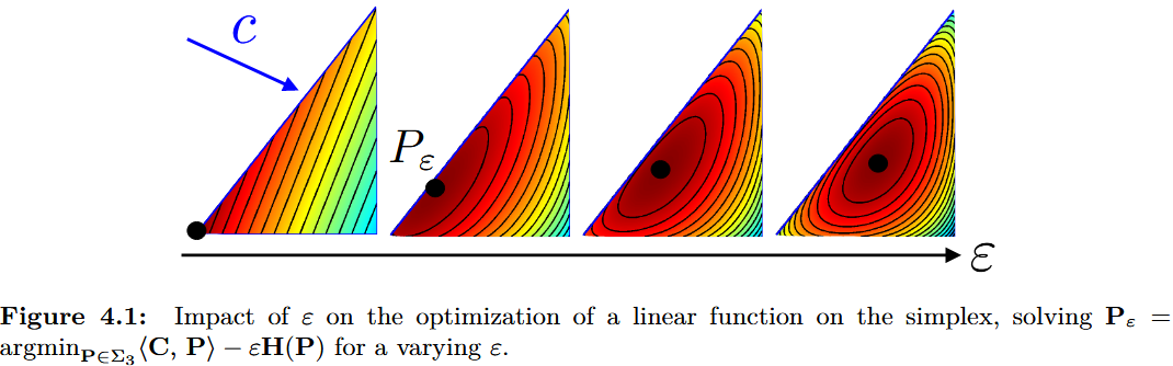
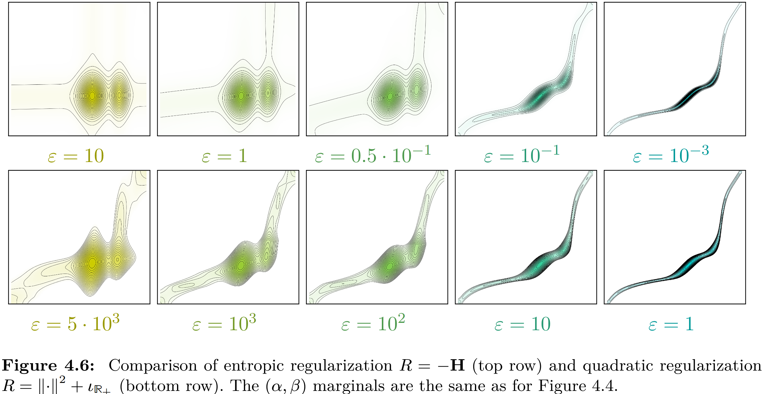
Seen on the coupling matrix, entropic regularization penalizes sparse plans made of a few high-flow paths and favors spreading the mass over many low-flow paths. The larger \(\varepsilon\), the blurrier and more spread out the coupling (it tends to \(\mathbf{a}\mathbf{b}^{\mathrm{T}}\) as \(\varepsilon\to\infty\)); the smaller \(\varepsilon\), the closer it gets to the sparse exact solution.
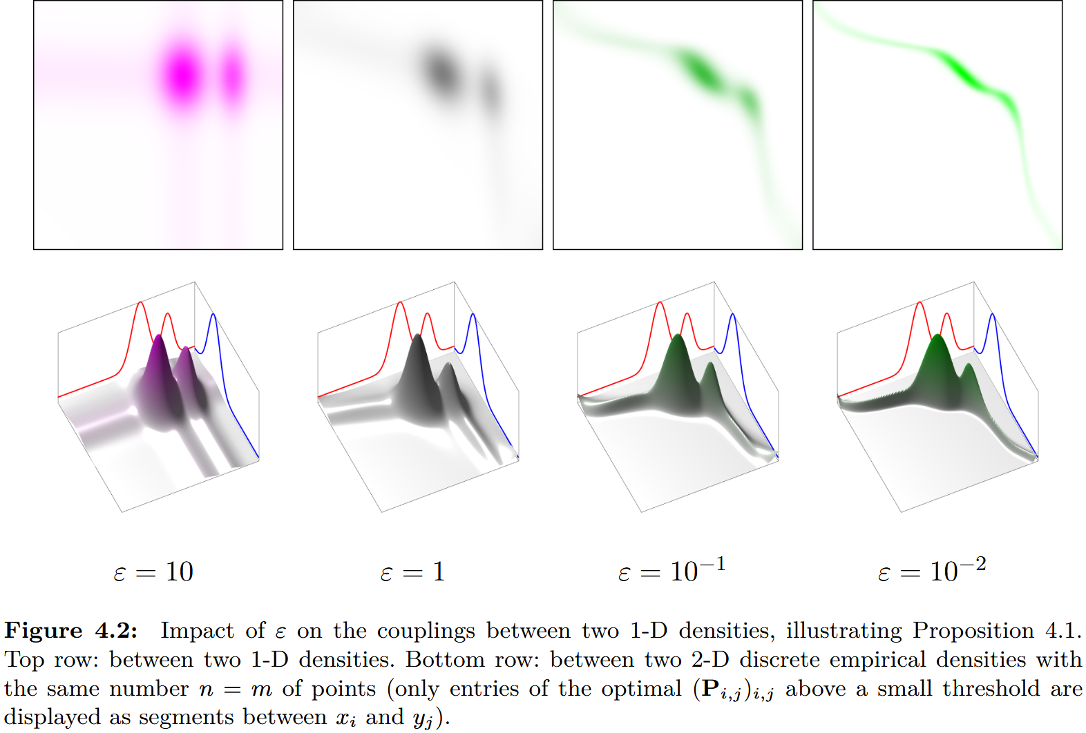
With the entropy term, the objective becomes strongly convex and the optimal solution has a very simple structure, which the Sinkhorn iterations in the next section exploit. That is why entropic regularization cuts the cost so much.
Aside: quadratic regularization. Besides entropy, one can also regularize with the quadratic term \(\|\mathbf{P}\|^2\). Its main advantage over entropy is that the optimal coupling is a sparse approximation, but the solvers are slower and cannot be parallelized as efficiently as Sinkhorn to compute many OT problems at once. In the figure below, the top row is entropic and the bottom row is quadratic:
3.3 The Sinkhorn algorithm
Sinkhorn is exactly the algorithm for the entropic problem above: one can show that the optimal solution always has the form \(\operatorname{diag}(u)\,K\,\operatorname{diag}(v)\), so all we need is to alternately rescale two vectors \(u\) and \(v\) until the row and column sums match the two marginals. Once we have \(u\) and \(v\), we have the optimal coupling of the regularized problem, which approximates the original one. Below we follow Cuturi (2013) through the derivation.
3.3.1 Notation
\(r\) and \(c\) are two probability vectors in the simplex \(\Sigma_d:=\{x\in \mathbb{R}_{+}^{d}: x^{\mathrm{T}}\mathbf{1}_d=1\}\). The transport polytope is
\[U(r, c) \stackrel{\text{def.}}{=}\left\{P \in \mathbb{R}_{+}^{d \times d}: P \mathbf{1}_d=r \quad \text{and} \quad P^{\mathrm{T}} \mathbf{1}_d=c\right\}\]\(P\) can be read as a joint distribution whose marginals are \(r\) and \(c\). \(M\) is the cost matrix; the paper takes it to be a distance matrix (zero on the diagonal and satisfying the triangle inequality):
\[\mathcal{M}=\left\{M \in \mathbb{R}_{+}^{d \times d}: \forall i, j \leq d,\ m_{ij}=0 \Leftrightarrow i=j,\quad \forall i, j, k \leq d,\ m_{ij} \leq m_{ik}+m_{kj}\right\}\]The objective is
\[d_{M}(r, c):=\min_{P \in U(r, c)}\langle P, M\rangle\]3.3.2 Sinkhorn distances
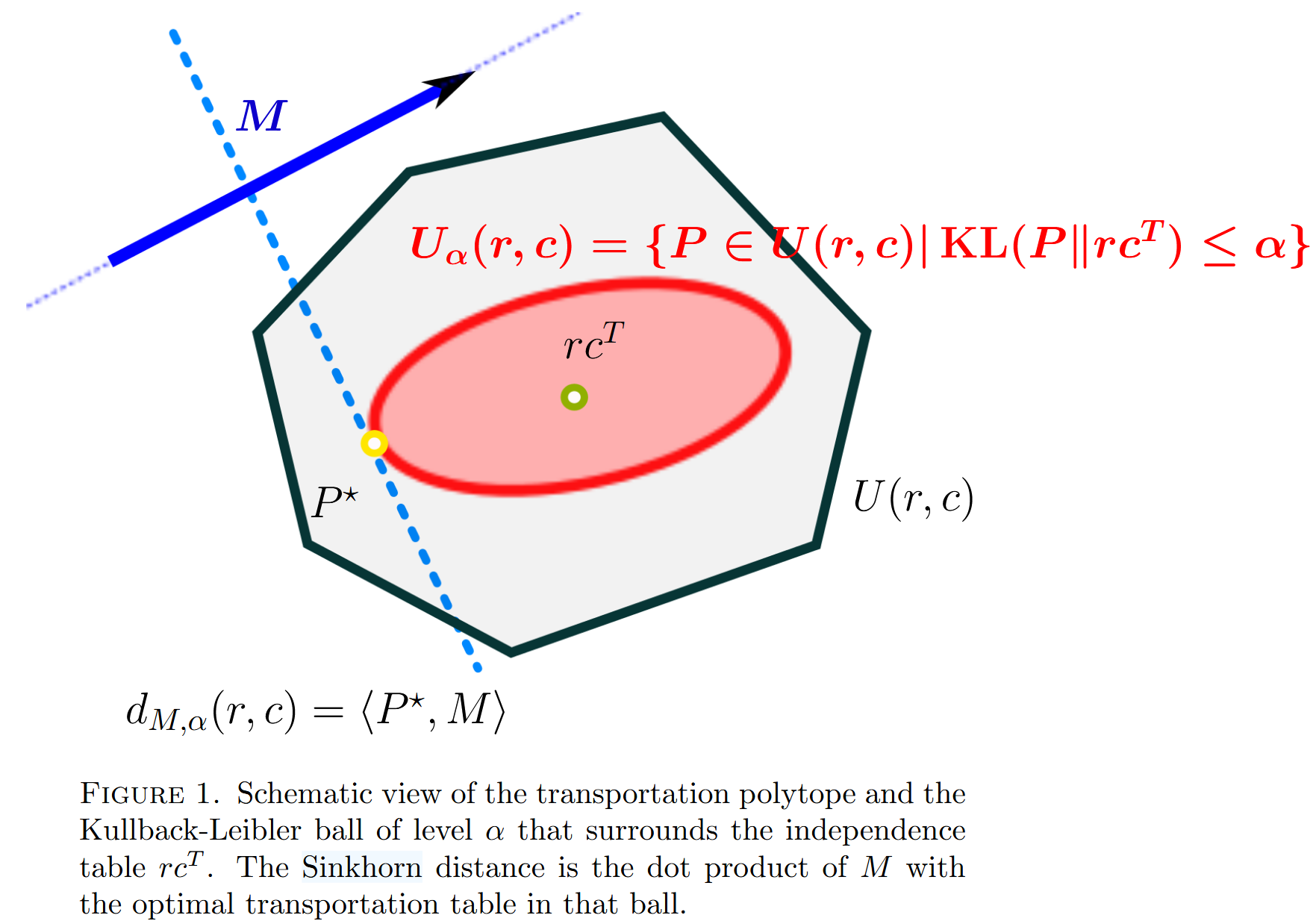
The idea is the same as before: to make the solution less sparse, increase its entropy. The coupling with the largest entropy in \(U(r,c)\) is the independent coupling \(rc^{\mathrm{T}}\): every entry is \(r_i c_j\), all strictly positive as long as \(r\) and \(c\) are, so it is the “densest” possible plan.
So we add a constraint that keeps \(P\) from straying too far from \(rc^{\mathrm{T}}\):
\[U_{\alpha}(r, c)=\left\{P \in U(r, c) \mid \mathrm{KL}\left(P \,\|\, r c^{\mathrm{T}}\right) \leq \alpha\right\}\]and define the Sinkhorn distance
\[d_{M, \alpha}(r, c) \stackrel{\text{def.}}{=} \min_{P \in U_{\alpha}(r, c)}\langle P, M\rangle\]As the figure shows, the Sinkhorn distance is the inner product of \(M\) with the optimal transport plan inside this KL ball.
A classic inequality from information theory (Cover & Thomas, 1991) says that the joint entropy never exceeds the sum of the marginal entropies:
\[\forall r, c \in \Sigma_{d},\ \forall P \in U(r, c), \quad h(P) \leq h(r)+h(c)\]Expanding the KL divergence then gives
\[U_{\alpha}(r, c)=\left\{P \in U(r, c) \mid h(P) \geq h(r)+h(c)-\alpha\right\} \subset U(r, c)\]We now prove the identity used here:
\[\mathrm{KL}\left(P \,\|\, r c^{\mathrm{T}}\right)=h(r)+h(c)-h(P)\]The KL divergence, entropy, and cross-entropy are defined as
\[\mathrm{KL}(P\|Q)=\sum_i P_i\log\frac{P_i}{Q_i}, \quad h(P)=-\sum_i P_i\log P_i, \quad H(P,Q) = -\sum_i P_i\log Q_i\]and \(\mathrm{KL}(P\|Q)=H(P,Q)-h(P)\). So it suffices to show that \(H(P,rc^{\mathrm{T}})=h(r)+h(c)\):
\[\begin{aligned} H(P,rc^{\mathrm{T}}) &= -\sum_{i,j}p_{ij}\log(r_i c_j) \\ &= -\sum_i\Big(\sum_j p_{ij}\Big)\log r_i-\sum_j\Big(\sum_i p_{ij}\Big)\log c_j \\ &= -\sum_i r_i\log r_i-\sum_j c_j\log c_j \\ &= h(r)+h(c) \end{aligned}\]The third step uses that the rows of \(P\) sum to \(r\) and its columns to \(c\). ∎
Back to the constraint \(h(P) \geq h(r)+h(c)-\alpha\): \(h(r)\) and \(h(c)\) are constants, so the constraint just says that \(h(P)\) is at least some constant. By Lagrangian duality, for every \(\alpha\) there is a \(\lambda>0\) such that the constrained problem is equivalent to minimizing
\[\langle P, M\rangle-\frac{1}{\lambda} h(P)\]i.e. we want \(h(P)\) to be as large as possible. This is the same problem as the entropic regularization in Section 3.2 (with \(\lambda = 1/\varepsilon\); the two entropies differ only by a constant).
Adding the marginal constraints, the Lagrangian is
\[L(P, \alpha, \beta)=\sum_{i,j} \Big(\frac{1}{\lambda} p_{ij} \log p_{ij}+p_{ij} m_{ij}\Big)+\alpha^{\mathrm{T}}\left(P \mathbf{1}_{d}-r\right)+\beta^{\mathrm{T}}\left(P^{\mathrm{T}} \mathbf{1}_{d}-c\right)\]Setting the partial derivative with respect to \(p_{ij}\) to zero:
\[\begin{aligned} \frac{1}{\lambda}(\log p_{ij}+1)+m_{ij}+\alpha_{i}+\beta_{j}&=0 \\ \log p_{ij}&=-1-\lambda(m_{ij}+\alpha_{i}+\beta_{j}) \\ p_{ij}^{\lambda}&=e^{-\frac{1}{2}-\lambda \alpha_{i}}\; e^{-\lambda m_{ij}}\; e^{-\frac{1}{2}-\lambda \beta_{j}} \end{aligned}\]Let \(u_{i}=e^{-\frac{1}{2}-\lambda \alpha_{i}}\), \(v_{j}=e^{-\frac{1}{2}-\lambda \beta_{j}}\), and \(K_{ij}=e^{-\lambda m_{ij}}\). In matrix form this is
\[P^{\lambda}=\operatorname{diag}(u)\, K\, \operatorname{diag}(v)\]So the only unknowns are \(u\) and \(v\). Plugging into the marginal constraints:
\[\sum_{j} p_{ij}=u_{i}\,(Kv)_{i}=r_{i}, \qquad \sum_{i} p_{ij}=v_{j}\,(K^{\mathrm{T}}u)_{j}=c_{j}\]This gives the update rules for \(u\) and \(v\), applied alternately as a fixed-point iteration until convergence:
\[u_{i}^{(t+1)}=\frac{r_{i}}{\big(K v^{(t)}\big)_{i}}, \qquad v_{j}^{(t+1)}=\frac{c_{j}}{\big(K^{\mathrm{T}} u^{(t+1)}\big)_{j}}\]Each step is just a matrix–vector product plus an element-wise division, which makes it well suited to batched computation on GPUs, and the iteration can be shown to converge linearly.
4. OT in practice
4.1 Wasserstein GAN (ICML 2017)
Replaces the JS divergence in the original GAN objective with the Wasserstein-1 distance (via Kantorovich–Rubinstein duality). When the supports of the two distributions barely overlap, the JS divergence gives vanishing gradients, while the Wasserstein distance still provides meaningful ones, so training is more stable.
4.2 Missing-data imputation with OT (ICML 2020)
Combines the Wasserstein distance, entropic regularization, and the Sinkhorn algorithm. The core idea: two batches drawn at random from the same dataset should come from the same distribution, so the Sinkhorn divergence between them should be small. Treating the missing values as optimization variables and minimizing the Sinkhorn divergence between batches gives the imputed values.
4.3 Neural Optimal Transport (ICLR 2023 Spotlight)
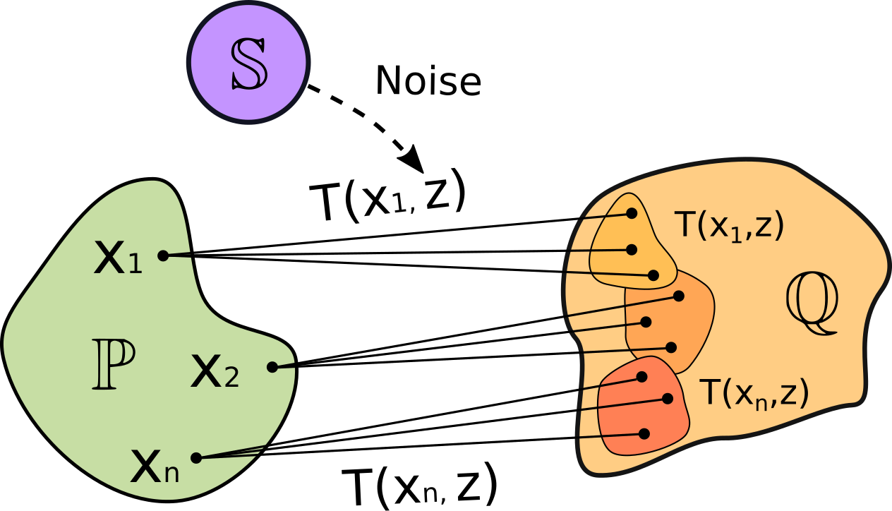
Learns a stochastic OT map \(T(x, z)\) with neural networks: the same input \(x\) combined with different noise \(z\) can map to multiple samples of the target distribution. This enables both one-to-one and one-to-many transfer, with a parameter that controls the diversity of the outputs. Code: iamalexkorotin/NeuralOptimalTransport.
References
- G. Peyré, M. Cuturi. Computational Optimal Transport. Foundations and Trends in Machine Learning, 2019.
- M. Cuturi. Sinkhorn Distances: Lightspeed Computation of Optimal Transport. NeurIPS, 2013.
- T. M. Cover, J. A. Thomas. Elements of Information Theory. Wiley, 1991.
- M. Arjovsky, S. Chintala, L. Bottou. Wasserstein Generative Adversarial Networks. ICML, 2017.
- B. Muzellec, J. Josse, C. Boyer, M. Cuturi. Missing Data Imputation using Optimal Transport. ICML, 2020.
- A. Korotin, D. Selikhanovych, E. Burnaev. Neural Optimal Transport. ICLR, 2023.