The post first explains why teleoperation needs haptic feedback and how humans perceive touch. It then reviews the ways haptic feedback can be rendered, grouped into vibration, force, electrical stimulation, shape arrays, and others. Next, it looks at several teleoperation systems, as well as UMI-style wearable data collection devices. It closes with a summary and discussion.

1. Why Teleoperation Needs Haptic Feedback

The performance of imitation learning depends heavily on data, yet what counts as “good data” is hard to define. Teleoperation is currently the main way to collect data for dexterous hands, and there are three common approaches:

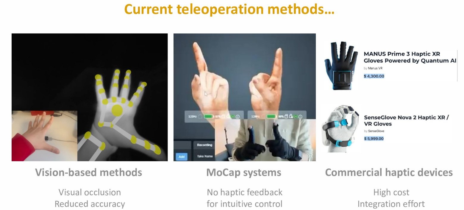
• Vision-based hand tracking (e.g., hand tracking on a VR headset): nothing to wear, but prone to occlusion and limited in accuracy;
• Motion-capture gloves: accurate, but the operator cannot feel the robot hand’s contacts and has to judge by sight whether it is touching something and how hard;
• Commercial haptic gloves (e.g., the force-feedback models from SenseGlove and MANUS): good feedback, but expensive and a lot of work to integrate with a robot system.

Without touch, the operator can only judge contact by sight. When the object is hidden behind the fingers, the contact force is small, or the grip force has to be controlled, this judgment is unreliable. A direct response is to build a low-cost device that combines motion capture with haptic and force feedback.

2. Human Tactile Perception

2.1 Four Types of Mechanoreceptors

The skin of the hand contains four main types of mechanoreceptors, each responsible for a different kind of tactile information:

This table serves as a reference for the rest of the post: which receptors a haptic device can stimulate determines what information it can convey. Vibration motors mainly stimulate Pacinian and Meissner corpuscles, so they are good at conveying contact and impacts. Conveying shape requires an array that stimulates Merkel discs, and conveying shear or pulling requires stretching the skin.

2.2 Haptic Feedback on Different Body Parts

Haptics is a major research topic in human–computer interaction (HCI). Long before the rise of embodied AI, a large body of HCI work studied how to let people feel virtual or remote environments. By body part, common targets include:

• Neck: simulating impacts to the head, and in some work guiding head rotation. Electrical muscle stimulation (EMS) is common here: electrodes placed on the relevant muscles make them contract, producing a sense of pressure or impact.
• Chest and back: usually a wearable vest with an array of vibration motors or mechanical pushers. When a collision happens in VR, the actuator at the matching location moves, producing a sense of pressure and impact.
• Arm: less studied; a typical approach uses EMS on the arm muscles to simulate the resistance of lifting a heavy object.
• Fingers: the most studied, with approaches ranging from vibration and electrotactile feedback to flexible electronic skin and microfluidics (Section 3).
• Whole body: for example, transcranial magnetic stimulation of the brain can produce touch sensations across many body parts (Section 3.3).

Teleoperation is mostly concerned with the fingers, but touch on the arm and torso is also useful, for instance to warn the operator that the robot arm is about to hit an obstacle (Section 4.4).

3. Ways to Render Haptic Feedback

3.1 Vibration: ERM, LRA, and Piezo

Vibration is the cheapest and most widely used form of haptic feedback, found in phones and game controllers. There are three common types of actuators:

• ERM (eccentric rotating mass): a DC motor with an off-center weight that vibrates as it spins. It is simple and very cheap, but amplitude and frequency are both set by the rotation speed and cannot be controlled independently, and it starts and stops slowly, so it can only produce a fairly coarse buzz. In consumer electronics it has largely been replaced by the LRA.
• LRA (linear resonant actuator): a coil, a magnet, and a spring, driven by an AC signal near the resonant frequency so that a mass moves back and forth. It responds quickly, uses little power, and produces a crisp vibration, which makes it the standard choice in current phones. Its drawback is that it is only efficient near the resonant frequency, so its bandwidth is narrow. By vibration direction, LRAs come in a vertical type (Z-axis, usually round) and a lateral type (X/Y-axis, usually rectangular, with a longer stroke and richer vibration).
• Piezo: the piezoelectric effect works both ways. Pressing on the material produces a voltage (the direct piezoelectric effect), which can be used for sensing; conversely, applying a voltage deforms the material (the converse piezoelectric effect), so driving it with AC makes it vibrate. Piezo actuators use the latter: piezo films or stacked ceramics deform at high frequency, giving the widest bandwidth and fastest response. They can be programmed to produce different sensations and are well suited to rendering texture and friction, but they need drive voltages of a hundred volts or more, which makes the drive circuitry and packaging more complex. Piezo should not be confused with piezoresistive materials, whose resistance merely changes with deformation: they can only be used for sensing, not actuation.

Recommended choices for different applications:

The limits of vibration are also clear: it can only convey whether there is contact and how strong it is, not shape, softness, or the direction of force.

3.2 Force Feedback

Force feedback aims to apply real resistance to the operator’s fingers, so that they feel the reaction force of grasping an object. Common structures include:

• Cable-driven: motors pull the fingers through cables; DOGlove uses this design (Section 4.1). It is light, but can only pull in one direction.
• Linkage exoskeleton: linkages transmit motor torque to each finger joint and can measure joint angles at the same time. Many data gloves follow this approach.
• Brakes / damping: instead of applying force actively, the device locks a joint or increases damping when needed. For example, ELAXO from Hsin-Ruey Tsai’s group uses adjustable resistance to render grasping and twisting, and DextrEMS (Section 3.3) also uses mechanical brakes. Passive designs are safe and power-efficient.

These structures also allow some simple extensions, such as adding pushers on both sides of a finger to introduce a lateral degree of freedom and convey shear force, or using dynamically adjustable damping to render the softness of an object.

Note that when force feedback is produced by motors, how it feels depends heavily on the control scheme. DOGlove found that simply raising the PID gain of the servos makes the feedback feel overly stiff and unnatural.

3.3 Electrical and Magnetic Stimulation

Electrical stimulation is very common in HCI research, and Pedro Lopes (now at the University of Chicago) has done a great deal of work in this area.

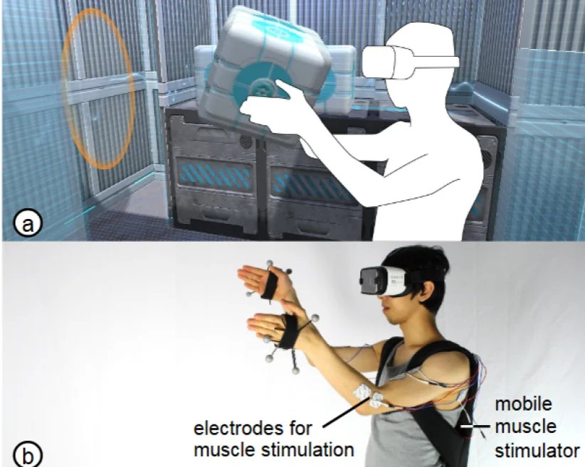
Electrical muscle stimulation (EMS) makes muscles contract involuntarily, producing a sense of being pushed back. For example, stimulating the arm muscles when the user pushes a wall or lifts a heavy box in VR makes the wall feel immovable and the box feel heavy:

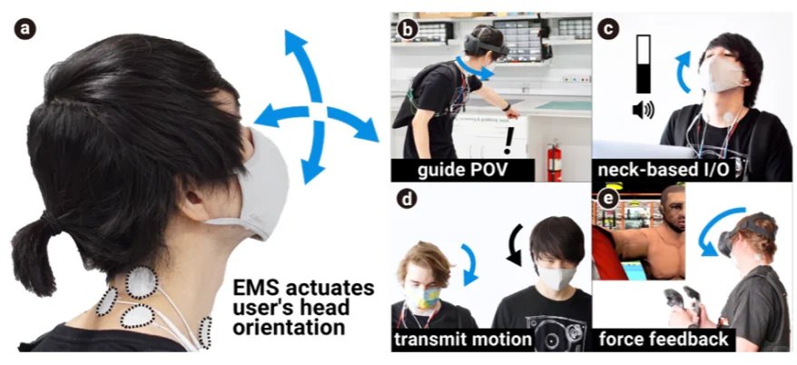
The same method can stimulate the neck muscles to turn the head directly and guide the user’s gaze:

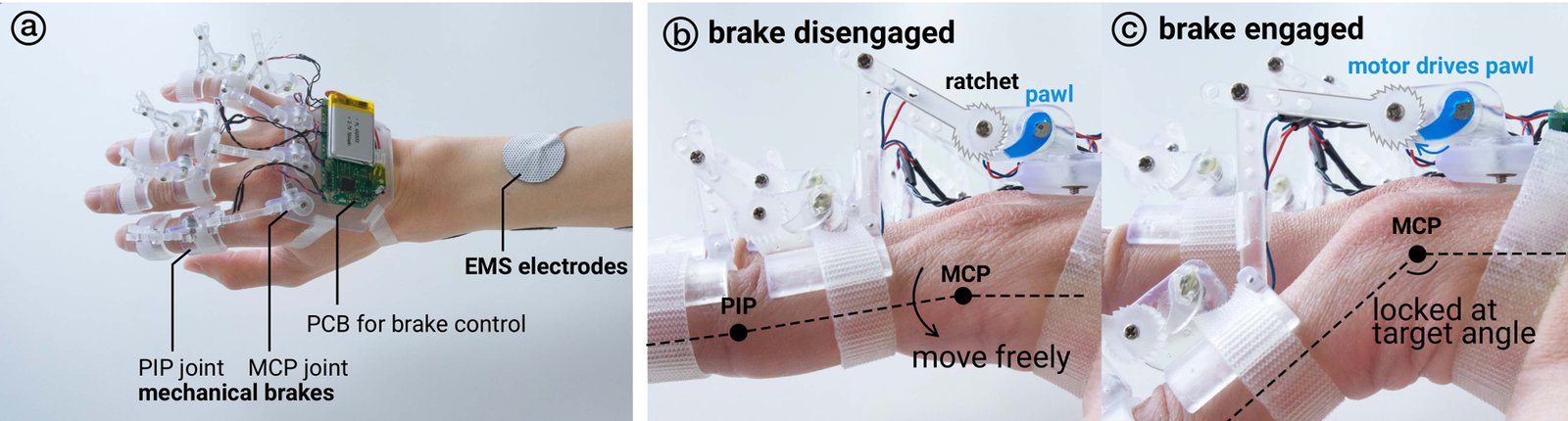
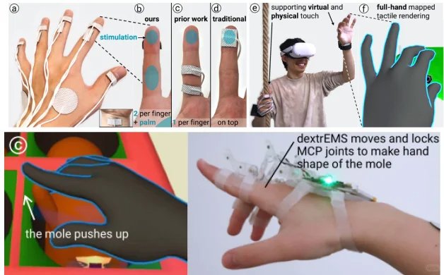
DextrEMS addresses two inherent problems of EMS: stimulating one finger also moves the others, and holding a finger still requires continuously contracting the opposing muscles, which makes the finger oscillate. It adds mechanical brakes to 8 finger joints (68 g in total): EMS actuates the fingers and the brakes lock them at the target position, enabling more dexterous control.

Full-hand electrotactile feedback without obstructing the palm (CHI 2023 Best Paper): electrodes are placed only on the back of the hand and the wrist. By stimulating the median and ulnar nerves, the device produces touch sensations at 11 locations on the palmar side. Since nothing covers the palm, the user can still grasp real objects normally.

Magnetic stimulation: the electrical pulses of EMS cause a tingling sensation, and EMS relies on pre-gelled electrodes that must stay in contact with the skin and dry out quickly. Stimulating muscles with magnetic fields instead (UIST 2023) reduces the tingling and works through clothing.

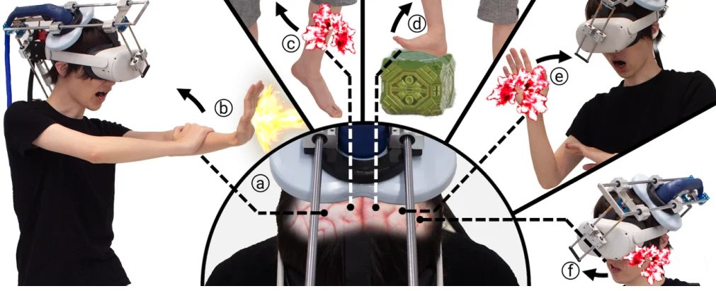
Haptic Source-Effector (CHI 2024) goes further: it applies transcranial magnetic stimulation (TMS) to the brain. Moving a single magnetic coil to different locations on the scalp produces 15 different touch and force sensations across the body, without placing an actuator on each body part.

The advantage of electrical (and magnetic) stimulation is that the devices can be very small and light while still producing real forces. Its limitations are equally clear: responses vary greatly between individuals, so calibration is needed before every use, and the tingling and safety risks make long sessions difficult. Overall, electrical stimulation remains mainly a research technique and is still far from a product suitable for long-term use.

3.4 Shape Arrays

Rendering shape requires a “pixel array” on the fingertip whose pixels can rise independently. The most direct approach is an array of mechanical pins, but it is hard to miniaturize; large tabletop pin arrays have also been built.

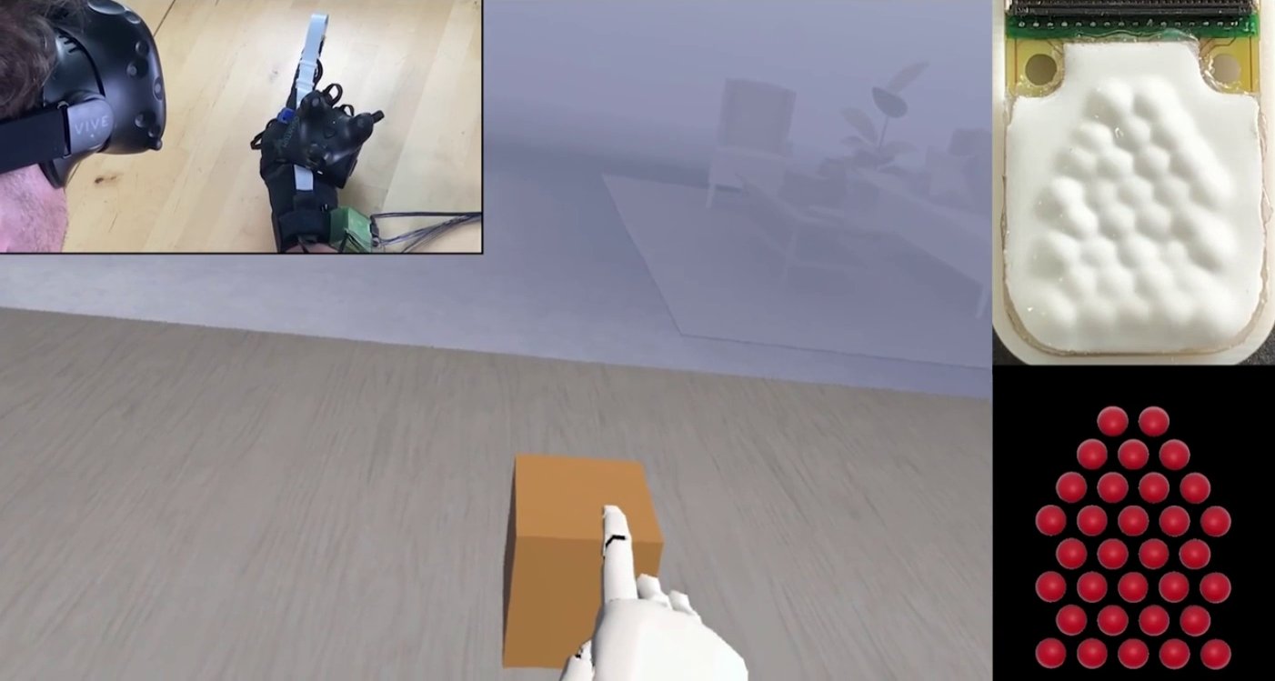
Fluid Reality (CMU, UIST 2023) is the closest to an ideal solution among the work covered here. Each fingertip carries an array of bubble-like pixels filled with liquid; when a pixel is energized, liquid flows into the bubble and inflates it. Each pixel is an electroosmotic pump only a few hundred micrometers thick, with no moving parts, which moves the liquid by acting directly on the charges in it with an electric field.

This design meets the requirements above well:

1. It is an array: it can convey the rough shape of an object and responds quickly;
2. It is cheap and portable: the glove is untethered and weighs only 207 g including all drive electronics and the battery, reportedly runs for about 3 hours, and costs under $1,000 to build.

The difficulty is fabrication: the packaging leaks easily, and improving on the design requires some background in chemistry (according to a fellow student who tried to reproduce it). The project has since been spun out into a company, so if the goal is a product, buying it may be more practical than reproducing it.

Flexible electronic skin and micro-vibration arrays can also render fine patterns and textures. They are safer than electrical stimulation and feel more realistic, but are similarly complex to fabricate.

3.5 Softness, Friction, and Other Sensations

Other work does not apply force directly, but instead changes how the finger perceives real objects:

• Altering perceived softness (Lopes’s group, UIST 2021 Best Paper): restricting the deformation of the fingerpad makes a rigid object feel softer. The device only clamps the sides of the fingerpad, leaving most of it exposed, so the user can still feel the object’s texture, and the object itself needs no modification.
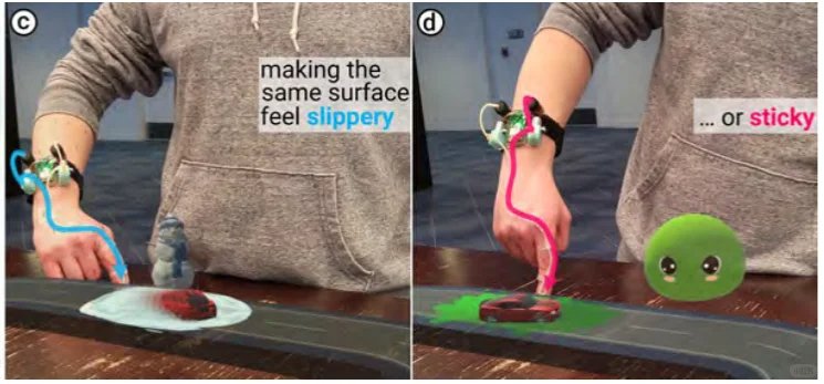
• Stick&Slip (Lopes’s group, CHI 2024): depositing a quickly evaporating liquid on the fingerpad changes the friction between the fingerpad and a surface, making the surface feel slippery or sticky (by about ±60%); friction returns to normal once the liquid evaporates. It does not require modifying the touched surface, but it only works when the finger touches a real surface, so it is hard to apply directly to teleoperation.

• HairTouch (CHI 2021): a bundle of brush hairs extends from a VR controller; changing how far the hairs extend and how tightly they are constrained renders differences in stiffness, roughness, and surface height.
• GuideBand (CHI 2021): three motors pull a wristband through strings, applying forces of different strengths in three dimensions to guide the forearm.
• FingerX (CHI 2022): extendable and withdrawable supports on the fingers work together with real objects to render the shapes of virtual objects.

Hsin-Ruey Tsai was involved in all three, and ELAXO, mentioned above, also comes from his lab.

Temperature and humidity are also part of touch, but they are hard to use in teleoperation: heat and liquid transfer too slowly to keep up with rapid changes in contact. Texture also has few applications, since in most manipulation tasks it has little effect on the motion.

3.6 Summary

4. Haptic Feedback in Teleoperation

4.1 DOGlove: A Low-Cost Haptic Force-Feedback Glove

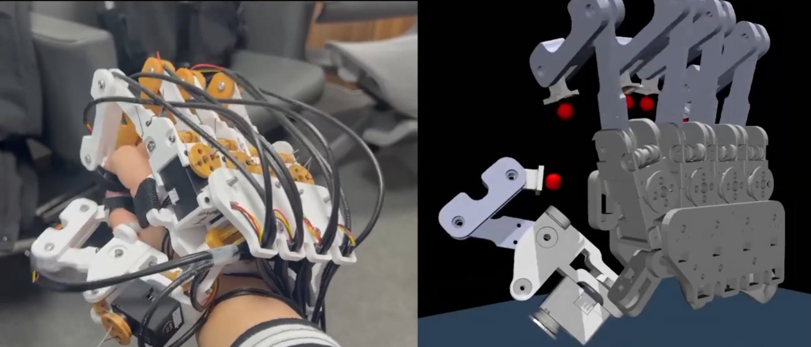
The goal of DOGlove (RSS 2025) is summed up in one line from its authors: “Bring everything about touch back to human.” It targets real-time teleoperation rather than offline demonstration, aiming for a low-cost device that combines motion capture with haptic and force feedback.

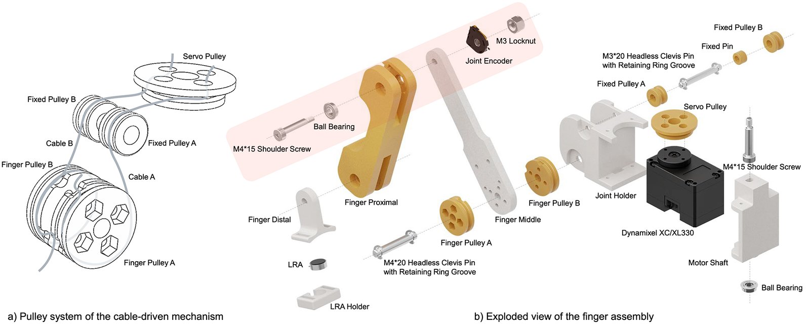
Hardware: 21-DoF motion capture plus 5-DoF force feedback, for a total cost under $600, and fully open source. Each finger is pulled by a motor through a cable to provide force feedback, and each fingertip has an LRA for vibration feedback.

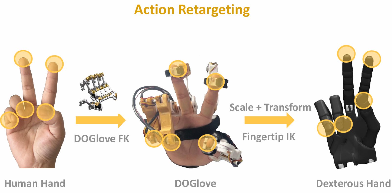
Action retargeting: the human hand and the robot hand differ in size and joint structure, so the joint angles measured by the glove have to be mapped onto the robot hand. DOGlove first computes the human fingertip positions with the glove’s forward kinematics, scales and transforms them, and then solves for the robot hand’s joint angles with its inverse kinematics. A key requirement is preserving finger opposition: when the human thumb and index finger touch, the robot’s thumb and index finger must touch as well. This mapping has to be designed by hand and takes considerable effort.

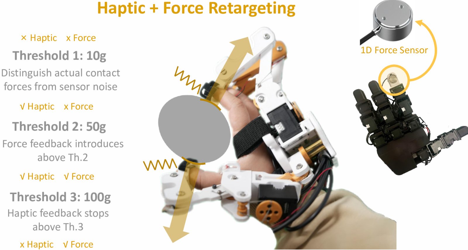
Haptic and force retargeting: the robot fingertips carry 1-D force sensors, and DOGlove switches between vibration and force feedback based on the measured force:

Force feedback is not used for light contact for two reasons. First, people are sensitive to vibration, so vibration conveys light contact more naturally. Second, force feedback is produced by adjusting the servo torque (specifically, the PID gain Kp), which tends to feel overly stiff at small forces.

Future directions: the authors argue that a binary or 1-D signal is not enough. Beyond whether contact happens, information such as material, softness, and temperature also matters, and they are experimenting with a shape-sensing array.

4.2 Bunny-VisionPro: Low-Cost Feedback with ERMs

Bunny-VisionPro (IROS 2025) uses the Apple Vision Pro for bimanual dexterous teleoperation and implements low-cost haptic feedback with ERMs:

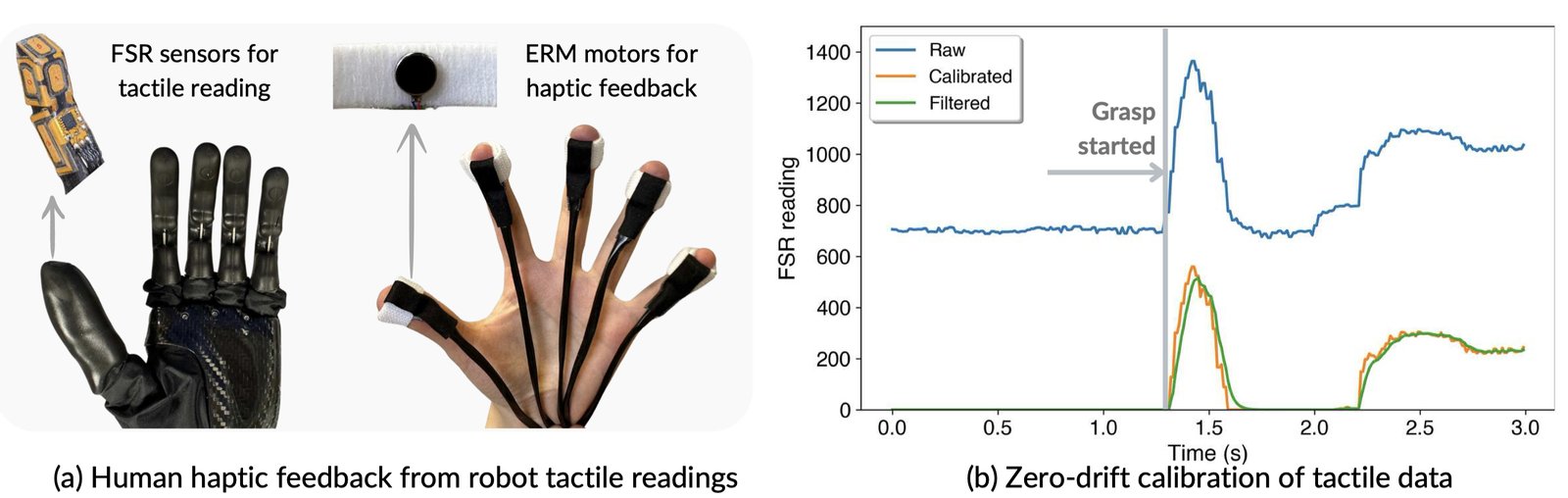
• FSR pressure sensors on the robot’s five fingertips read the contact pressure between the fingers and the object in real time;
• the readings are zero-calibrated (baselines are collected at multiple joint positions, interpolated, and subtracted) and then low-pass filtered;
• the tactile intensity is normalized to a 0–255 PWM duty cycle that directly drives ERM vibration motors on the operator’s fingers.

The paper also adds touch to the policy input in two ways: as a vector appended to the robot state and encoded with an MLP, and as points, where fingertips in contact are added to the camera point cloud for visual encoding. The results:

• in simple single-arm tasks, tactile input brings almost no improvement;
• in bimanual tasks (such as bimanual pinching and cooperative carrying), it brings a small improvement;
• a user study shows that operators subjectively prefer having vibration feedback, finding it more natural and making contact easier to perceive.

This suggests that haptic feedback may help the person collecting the data more directly than it helps the policy as an input. In addition, ERMs are rather dated, and switching to LRAs would give better feedback.

4.3 Visualizing Touch in AR

Besides delivering touch to the hand, another approach is to visualize tactile information:

• The teleoperation system TactAR in RDP (Reactive Diffusion Policy, RSS 2025) renders tactile and force-induced deformation on the end effector in AR in real time, helping the operator with tasks that require controlling contact force, such as peeling a cucumber or wiping writing off a vase;
• A dexterous-hand work from KTH (Learning Dexterous In-Hand Manipulation with Multifingered Hands via Visuomotor Diffusion, IROS 2025) tracks the human hand with Meta Quest 3 passthrough AR and overlays the tracking result, so the operator can see the hand pose in real time; it provides no haptic feedback.

Building on this, the direction of force and the contact locations could also be overlaid in AR. RDP uses a gripper; extending it to a dexterous hand and overlaying the tactile visualization directly on the operator’s own hand may work even better.

4.4 Whole-Body Vibrotactile Cues

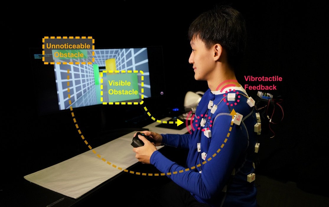
AeroHaptix is a wearable vibrotactile system: when the operator flies a drone remotely, obstacles that are not visible on screen are signaled by vibrations at the corresponding location on the body, reducing collisions.

The same idea applies to robot teleoperation: a few vibration motors on the operator’s arm or torso could warn that the robot arm is about to hit something nearby. Arm exoskeletons (such as AirExo) already exist, but using touch to signal collisions is still worth exploring.

5. UMI-Style Wearable Data Collection

UMI records human manipulation directly with a handheld gripper, with no robot needed during collection. The following works extend this idea to dexterous hands: the collection device is worn on the hand and people perform the task with their own hands, so they naturally have full tactile feedback and there is no need to render touch back to the operator.

5.1 Feel the Force: The Same Tactile Sensor on Hand and Gripper

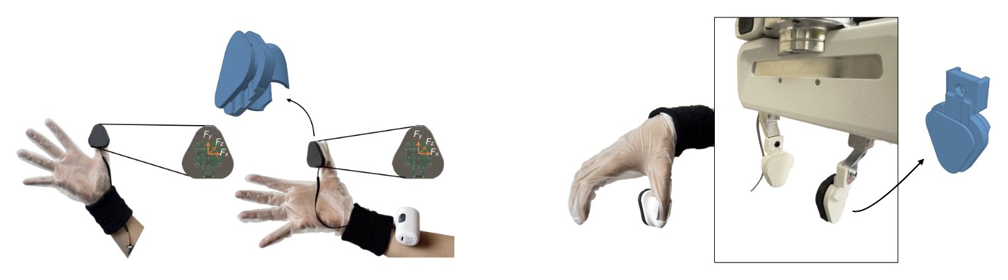
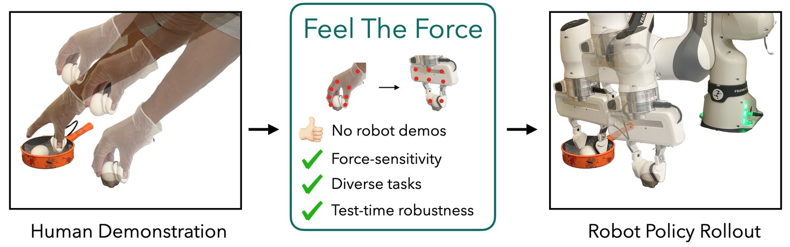
FTF (Feel the Force, RSS 2025 workshop) does not use teleoperation but collects human demonstrations directly. The operator wears a glove with an AnySkin-style magnetic tactile sensor on the thumb pad, and one fingertip of the robot gripper carries the same sensor. The idea is that if human forces are to be transferred to the robot, both ends should use the same sensor. For simplicity, the mapping from the human hand to the gripper is fixed.

The policy learns from the history of robot and object keypoint trajectories, forces, and gripper states, predicts future motion and the required contact force, and passes them to the gripper’s force feedback controller for execution.

5.2 DexUMI: An Exoskeleton Matching the Robot Hand’s Kinematics

DexUMI (CoRL 2025, Best Paper finalist) aims to close two gaps between the human hand and a dexterous robot hand:

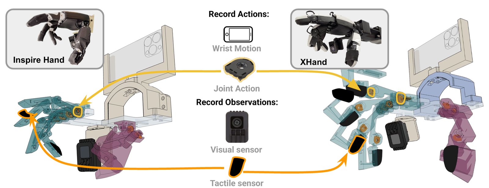
• Hardware gap: an exoskeleton is designed for a specific robot hand (such as the Inspire Hand or XHand), with joints and link lengths matching the robot hand. When a person operates while wearing it, the motion maps over directly, without retargeting.
• Visual gap: segmentation and image inpainting models remove the human hand and exoskeleton from the video and replace them with images of the robot hand, so the training data looks visually like the robot doing the task itself.

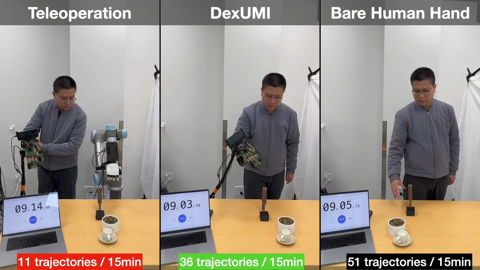
Compared with UMI, DexUMI is less novel, but it runs the full pipeline from data collection to policy deployment and collects data much more efficiently: in 15 minutes, teleoperation yields 11 trajectories, DexUMI 36, and the bare human hand 51.

5.3 DEXOP: A Hand Exoskeleton with a Passive Robot Hand

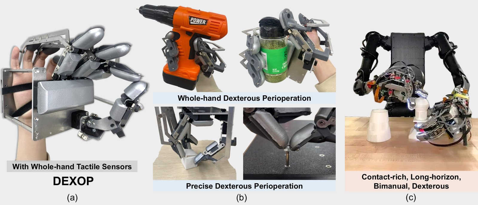
DEXOP proposes a collection paradigm called perioperation: the person wears a hand exoskeleton connected to a passive robot hand, and the human fingers drive the robot fingers directly through linkages, allowing 1:1 operation.

• Collection is fast, the operator feels contacts directly, and precision is ensured;
• the robot hand is covered with tactile sensors; although touch cannot fully capture shape, the operator can rely on sight, which ensures that the collected data completes the task;
• only a wrist camera and touch are used, with no third-person view, so no human hand appears in the images and there is no visual gap;
• the arm is mounted on the AirExo-2 whole-arm exoskeleton, so arm motion is collected at the same time.

Its limitations: the width of the linkages makes finger opposition difficult and causes some collisions. In addition, DEXOP is built around the authors’ own robot hand, designed from the start to be mounted and removed; a sealed commercial dexterous hand would be hard to modify in the same way.

5.4 Other Related Work

• DigituSync (UIST 2022): a passive exoskeleton that links two people’s hands, transmitting finger motion in real time with an adjustable force ratio between the two. The idea is close to DEXOP, but it only transmits finger flexion and cannot perform grasps.
• Festo ExoHand (2012): an early pneumatic exoskeleton hand that transmits human hand motion to a robot hand in real time and feeds the robot hand’s grasp force back to the operator, making it bidirectional.
• Embroidered smart gloves (Nature Communications 2024): a digital embroidery machine stitches piezoresistive tactile sensors and vibration actuators directly into fabric, quickly producing gloves that both sense and give feedback; the demonstrations include robot teleoperation.
• Open-source tactile sensors: for example, 3D-ViTac open-sourced a low-cost flexible tactile sensor that the authors say can be made in 30 minutes. Human-hand collection setups such as DexUMI currently cannot record touch; attaching such sensors to the hand would capture tactile data as well.
• Co-Embodiment: an experiment shown at a conference, later written up as the paper One Body, Two Minds (KTH, 2026). A diffusion policy handles grasping, and the user only needs to nod to trigger task-relevant finger actions, such as pressing a drill’s trigger. Users adapt to this control scheme quickly. This suggests that a low-DoF hand could perhaps be controlled with four buttons and a joystick, though less efficiently than with DEXOP.

6. Summary and Discussion

1. Electrical stimulation is the most common in research but hard to turn into a product. Individual differences are large, calibration is required before use, and there are safety risks, so it remains mainly a research technique.
2. Flexible skin, liquid pumps, and micro-vibration arrays are safer and feel more realistic, but are complex to fabricate.
3. High-fidelity touch is hard to achieve with any single technique and calls for interdisciplinary work. For embodied AI, the more sensible direction is to focus on embodied data rather than on haptics for its own sake: prioritize convenient, high-quality data collection over a high-fidelity collection experience.
4. When the scene is visible and control is easy, simple vibration feedback is largely sufficient. DOGlove essentially reaches the ceiling of simple haptic feedback; further gains mostly come from combining actuators such as ERMs and LRAs.
5. Sensor placement should be driven by collection needs, not by the designer’s assumptions. Whether to add sensing at the middle phalanges or control at the fingertips, for example, should depend on what is actually needed during collection.

In summary, touch plays three main roles in embodied data collection:

In my view, the third approach is the most scalable: the device is worn on the hand, collection is fast, and the operation matches human proprioception, making it the form of data collection closest to the human.

Finally, before collecting data, it may be worth first defining what good teleoperation data actually is: which of trajectories, velocities, and forces the policy really needs.

References

Teleoperation and Data Collection

1. H. Zhang, S. Hu, Z. Yuan, H. Xu. DOGlove: Dexterous Manipulation with a Low-Cost Open-Source Haptic Force Feedback Glove. RSS, 2025.
2. R. Ding, Y. Qin, J. Zhu, C. Jia, et al. Bunny-VisionPro: Real-Time Bimanual Dexterous Teleoperation for Imitation Learning. IROS, 2025.
3. A. Adeniji, Z. Chen, V. Liu, V. Pattabiraman, et al. Feel the Force: Contact-Driven Learning from Humans. arXiv, 2025.
4. R. Bhirangi, V. Pattabiraman, E. Erciyes, Y. Cao, et al. AnySkin: Plug-and-play Skin Sensing for Robotic Touch. ICRA, 2025.
5. C. Chi, Z. Xu, C. Pan, E. Cousineau, et al. Universal Manipulation Interface: In-The-Wild Robot Teaching Without In-The-Wild Robots. RSS, 2024.
6. M. Xu, H. Zhang, Y. Hou, Z. Xu, et al. DexUMI: Using Human Hand as the Universal Manipulation Interface for Dexterous Manipulation. CoRL, 2025.
7. H.-S. Fang, B. Romero, Y. Xie, A. Hu, et al. DEXOP: A Device for Robotic Transfer of Dexterous Human Manipulation. arXiv, 2025.
8. H. Fang, H.-S. Fang, Y. Wang, J. Ren, et al. AirExo: Low-Cost Exoskeletons for Learning Whole-Arm Manipulation in the Wild. ICRA, 2024.
9. H. Fang, C. Wang, Y. Wang, J. Chen, et al. AirExo-2: Scaling up Generalizable Robotic Imitation Learning with Low-Cost Exoskeletons. CoRL, 2025.
10. H. Xue, J. Ren, W. Chen, G. Zhang, et al. Reactive Diffusion Policy: Slow-Fast Visual-Tactile Policy Learning for Contact-Rich Manipulation. RSS, 2025.
11. P. Koczy, M. C. Welle, D. Kragic. Learning Dexterous In-Hand Manipulation with Multifingered Hands via Visuomotor Diffusion. IROS, 2025.
12. P. Koczy, Y. Zhang, D. Kragic, M. C. Welle. One Body, Two Minds: Variable Autonomy Approach for a Co-embodied Robotic Hand. arXiv, 2026.
13. B. Huang, Y. Wang, X. Yang, Y. Luo, Y. Li. 3D-ViTac: Learning Fine-Grained Manipulation with Visuo-Tactile Sensing. CoRL, 2024.
14. Y. Luo, C. Liu, Y. J. Lee, J. DelPreto, et al. Adaptive tactile interaction transfer via digitally embroidered smart gloves. Nature Communications, 2024.
15. B. Huang, Z. Wang, Q. Cheng, S. Ren, et al. AeroHaptix: A Wearable Vibrotactile Feedback System for Enhancing Collision Avoidance in UAV Teleoperation. IEEE RA-L, 2025.
16. Festo. ExoHand. Bionic Learning Network, 2012.

Haptic Feedback (HCI)

1. P. Lopes, S. You, L.-P. Cheng, S. Marwecki, P. Baudisch. Providing Haptics to Walls & Heavy Objects in Virtual Reality by Means of Electrical Muscle Stimulation. CHI, 2017.
2. Y. Tanaka, J. Nishida, P. Lopes. Electrical Head Actuation: Enabling Interactive Systems to Directly Manipulate Head Orientation. CHI, 2022.
3. R. Nith, S.-Y. Teng, P. Li, Y. Tao, P. Lopes. DextrEMS: Increasing Dexterity in Electrical Muscle Stimulation by Combining it with Brakes. UIST, 2021.
4. Y. Tanaka, A. Shen, A. Kong, P. Lopes. Full-hand Electro-Tactile Feedback without Obstructing Palmar Side of Hand. CHI, 2023.
5. Y. Tanaka, A. Takahashi, P. Lopes. Interactive Benefits from Switching Electrical to Magnetic Muscle Stimulation. UIST, 2023.
6. Y. Tanaka, J. Serfaty, P. Lopes. Haptic Source-effector: Full-body Haptics via Non-invasive Brain Stimulation. CHI, 2024.
7. Y. Tao, S.-Y. Teng, P. Lopes. Altering Perceived Softness of Real Rigid Objects by Restricting Fingerpad Deformation. UIST, 2021.
8. A. Mazursky, J. Serfaty, P. Lopes. Stick&Slip: Altering Fingerpad Friction via Liquid Coatings. CHI, 2024.
9. J. Nishida, Y. Tanaka, R. Nith, P. Lopes. DigituSync: A Dual-User Passive Exoskeleton Glove That Adaptively Shares Hand Gestures. UIST, 2022.
10. V. Shen, T. Rae-Grant, J. Mullenbach, C. Harrison, C. Shultz. Fluid Reality: High-Resolution, Untethered Haptic Gloves using Electroosmotic Pump Arrays. UIST, 2023.
11. Z.-Y. Zhang, H.-X. Chen, S.-H. Wang, H.-R. Tsai. ELAXO: Rendering Versatile Resistive Force Feedback for Fingers Grasping and Twisting. UIST, 2022.
12. H.-R. Tsai, C. Tsai, Y.-S. Liao, Y.-T. Chiang, Z.-Y. Zhang. FingerX: Rendering Haptic Shapes of Virtual Objects Augmented by Real Objects using Extendable and Withdrawable Supports on Fingers. CHI, 2022.
13. H.-R. Tsai, Y.-C. Chang, T.-Y. Wei, C.-A. Tsao, et al. GuideBand: Intuitive 3D Multilevel Force Guidance on a Wristband in Virtual Reality. CHI, 2021.
14. C.-J. Lee, H.-R. Tsai, B.-Y. Chen. HairTouch: Providing Stiffness, Roughness and Surface Height Differences Using Reconfigurable Brush Hairs on a VR Controller. CHI, 2021.

本文首先说明遥操作为什么需要触觉反馈，并介绍人体的触觉感知机制；随后按振动、力、电刺激、形状阵列等类别梳理触觉反馈的实现方式；接着分析几个具体的遥操作系统，以及类 UMI 的穿戴式采集装置；最后进行总结与讨论。

1. 遥操作为什么需要触觉反馈

模仿学习的效果在很大程度上取决于数据，但”什么是好的数据”很难定义。遥操作是目前采集灵巧手数据的主流方式，常见的有三类：

• 基于视觉的手势识别（如用 VR 头显追踪手部）：无需穿戴设备，但容易受遮挡影响，精度有限；
• 动作捕捉手套：精度高，但操作者感受不到机械手的接触，只能依靠视觉判断是否接触以及接触力的大小；
• 商用力触觉手套（如 SenseGlove、MANUS 的力反馈型号）：反馈效果好，但价格昂贵，且与机器人系统集成的工作量较大。

缺少触觉时，操作者只能依靠视觉判断接触状态。当物体被手指遮挡、接触力很小，或需要控制抓握力度时，这种判断并不可靠。因此，一个直接的思路是研制兼具动作捕捉和力触觉反馈、且成本较低的设备。

2. 人体的触觉感知

2.1 皮肤中的四类机械感受器

手部皮肤中主要有四类机械感受器，分别负责不同的触觉信息：

该表可作为后文讨论的参照：一种触觉反馈装置能刺激哪类感受器，决定了它能传递哪类信息。振动马达主要刺激环层小体和迈斯纳小体，因此适合表达接触和碰撞；表达形状需要能刺激默克尔触盘的阵列；表达剪切和拉扯则需要使皮肤产生拉伸。

2.2 不同身体部位的触觉反馈

触觉是人机交互（human–computer interaction，HCI）领域的重要研究方向。在具身智能兴起之前，已有大量 HCI 研究关注如何让人感知虚拟或远程环境。按身体部位划分，常见的有：

• 脖颈：模拟头部受到的撞击，也有工作用于引导头部转动。常用肌肉电刺激（EMS）：将电极贴在对应肌肉上，刺激肌肉收缩，从而产生压力或撞击感。
• 胸背：一般为穿戴式背心，其上排布多个振动马达或机械推杆，VR 中发生碰撞时，对应位置的装置动作，产生压力和碰撞感。
• 手臂：研究相对较少，典型做法是用 EMS 刺激手臂肌肉，模拟搬起重物时的阻力。
• 手指：研究最多，涉及振动、电触觉、柔性电子皮肤和微流体等方式，详见第 3 节。
• 全身：例如用经颅磁刺激作用于大脑，在全身多个部位产生触觉（3.3 节）。

遥操作主要关注手指，但手臂和躯干的触觉同样有用，例如提示操作者机械臂即将碰到障碍物（4.4 节）。

3. 触觉反馈的实现方式

3.1 振动：ERM、LRA 与压电

振动是成本最低、应用最广的触觉反馈方式，常见于手机和游戏手柄。常用的执行器有三类：

• ERM（Eccentric Rotating Mass，偏心转子马达）：带偏心配重的直流电机，旋转时产生振动。结构简单、成本极低，但振幅和频率都由转速决定，无法独立控制，启停也较慢，只能提供较粗糙的振感。在消费电子中已基本被 LRA 取代。
• LRA（Linear Resonant Actuator，线性马达）：由线圈、磁铁和弹簧组成，用交流信号在共振频率附近驱动质量块往复运动。响应快、功耗低、振感清晰，是目前手机的主流方案；缺点是只在共振频率附近效率较高，频带较窄。按振动方向可分为纵向（Z 轴，通常为圆形）和横向（X/Y 轴，通常为长方形，行程更大，振感更丰富）两种。
• 压电（piezo）：压电效应是双向的。材料受压时产生电压（正压电效应），可用于传感；反之，施加电压时材料发生形变（逆压电效应），以交流电驱动即可产生振动。压电执行器利用的是后者，用压电薄膜或叠层陶瓷在高频下形变，频带宽、响应最快，可以编程出不同的触感，适合模拟纹理和摩擦；但需要上百伏的驱动电压，驱动电路和封装都更复杂。需要与压阻区分：压阻材料只是电阻随形变变化，只能用于采集，不能用于驱动。

不同应用场景下的选型建议如下：

振动的局限同样明显：它只能表达是否接触以及接触的强弱，无法表达形状、软硬和力的方向。

3.2 力反馈

力反馈的目标是在操作者的手指上施加真实的阻力，使其感知到抓握物体时的反作用力。常见的结构有以下几种：

• 绳驱：电机通过绳索牵引手指，DOGlove 即采用这种方案（4.1 节）。结构轻，但只能提供单一方向的拉力。
• 连杆外骨骼：用连杆将电机的力矩传递到各个指节，同时可以测量关节角度，许多数据手套采用这一思路。
• 制动器 / 阻尼：不主动施力，而是在需要时锁住关节或增大阻尼。例如 Hsin-Ruey Tsai 组的 ELAXO 用可调阻力模拟抓握和扭转，DextrEMS（3.3 节）中也使用了机械制动器。被动式方案的优点是安全、省电。

在上述结构的基础上，还可以做一些简单的扩展，例如在手指两侧增加推杆，引入侧摆方向的自由度，从而传递剪切力的感觉；或者用动态可调的阻尼模拟物体的软硬。

需要注意的是，用电机实现力反馈时，反馈的主观感受在很大程度上取决于控制方式。DOGlove 的实践表明，若只是简单地增大伺服的 PID 增益，操作者会感到反馈过硬、不自然。

3.3 电刺激与磁刺激

电刺激在 HCI 研究中非常常见，Pedro Lopes（现任职于芝加哥大学）在这一方向做了大量工作。

肌肉电刺激（EMS） 使肌肉非自主地收缩，从而产生被推开的感觉。例如在 VR 中推墙或搬起重箱时刺激手臂肌肉，使人感到墙推不动、箱子很重：

同样的方法也可以用于刺激颈部肌肉，直接驱动头部转动，以引导视线：

DextrEMS 针对 EMS 的两个固有问题：刺激一根手指时，其他手指也会随之运动；要让手指保持静止，只能持续收缩对侧肌肉，导致手指上下振荡。该工作在 8 个指关节上加装了机械制动器（整套仅 68 克），由 EMS 负责驱动、制动器负责将手指锁定在目标位置，从而实现更灵巧的控制。

不遮挡手掌的全手电触觉（CHI 2023 最佳论文）：电极只贴在手背和手腕上，通过刺激正中神经和尺神经，使人在手掌一侧的 11 个位置感知到触觉。由于手掌侧没有任何装置，用户可以正常抓握真实物体。

磁刺激：EMS 的电脉冲会带来刺痛感，且依赖预先涂好凝胶的电极，电极需要贴紧皮肤，凝胶也很快会变干。改用磁场刺激肌肉（UIST 2023）可以减轻刺痛感，并能隔着衣物进行刺激。

Haptic Source-Effector（CHI 2024）更进一步：用经颅磁刺激（TMS）作用于大脑，将磁线圈移动到头皮上的不同位置，即可在全身产生 15 种不同的触觉和力觉，无需在每个部位都安装执行器。

电刺激（包括磁刺激）的优点是设备可以做得很小、很轻，并能产生真实的力。但其局限同样明显：不同个体对电刺激的反应差异很大，每次使用前都需要校准；刺痛感和安全风险也使其难以长时间使用。总体而言，电刺激目前主要停留在研究阶段，距离可长期使用的产品还有较大距离。

3.4 形状阵列

要表达形状，需要在指尖放置一个”像素阵列”，每个像素可以独立凸起。最直接的方案是机械推杆阵列，但难以小型化；桌面尺度的大型推杆阵列已有相关工作。

Fluid Reality（CMU，UIST 2023）是本次调研中最接近理想的方案。每个指尖有一个由气泡状像素组成的阵列，像素内装有液体，通电后液体流入气泡使其鼓起。每个像素都是一个仅几百微米厚的电渗泵，没有任何运动部件，直接利用电场驱动液体中的电荷流动。

该方案较好地兼顾了前述需求：

1. 具备阵列：可以表达物体的大致形状，且响应迅速；
2. 低成本、便携：整只手套无需连接外部设备，含全部驱动电路和电池仅 207 克，据报道续航约 3 小时，制作成本在 1000 美元以内。

其难点在于制作：封装容易漏液，在此基础上进行改进也需要一定的化学背景（据尝试复现的同学反馈）。该项目后来已成立公司，若以产品落地为目标，直接采购可能比自行复现更可行。

此外，柔性电子皮肤和微振动阵列也可以模拟精细的图案和纹理，比电刺激更安全、触感更真实，但工艺同样复杂。

3.5 软硬、摩擦及其他感觉

另有一些工作不直接施加力，而是改变手指对真实物体的感知：

• 改变软硬感（Lopes 组，UIST 2021 最佳论文）：通过限制指腹的形变，使硬质物体被感知为更软。装置只夹在指腹两侧，指腹大部分保持裸露，仍能感知物体的纹理，也无需改造物体本身。
• Stick&Slip（Lopes 组，CHI 2024）：在指腹上沉积一层快速蒸发的液体，改变指腹与表面之间的摩擦系数，使表面变滑或变黏（约 ±60%），液体蒸发后摩擦即恢复原状。该方法无需改造被触摸的表面，但前提是手指接触真实表面，因此难以直接用于遥操作。

• HairTouch（CHI 2021）：在 VR 手柄上伸出一束毛刷，通过改变毛发伸出的长度和约束程度，表达软硬、粗糙度和表面高度的差异。
• GuideBand（CHI 2021）：三个电机通过绳索牵引手腕上的腕带，在三维方向上施加不同强度的拉力，用于引导小臂的运动方向。
• FingerX（CHI 2022）：在手指上安装可伸出和收回的支撑结构，配合真实物体渲染虚拟物体的形状。

以上三项工作均有 Hsin-Ruey Tsai 参与，前文提到的 ELAXO 也出自其实验室。

温度和湿度同样属于触觉，但难以用于遥操作：热量和液体的传导过慢，无法跟上接触状态的快速变化。纹理的应用场景也较少，在大多数操作任务中，纹理对动作的影响并不明显。

3.6 小结

4. 遥操作中的触觉反馈

4.1 DOGlove：低成本的力触觉手套

DOGlove（RSS 2025）的目标可以用作者的一句话概括：”Bring everything about touch back to human.” 它面向实时遥操作而非离线示教，旨在实现兼具动作捕捉和力触觉反馈的低成本设备。

硬件：21 自由度的动作捕捉与 5 自由度的力反馈，整套成本低于 600 美元，并且开源。每根手指由电机通过绳索牵引，提供拉力反馈；每个指尖装有一个 LRA，提供振动反馈。

动作重定向（retargeting）：人手与灵巧手的尺寸和关节结构不同，需要将手套测得的关节角映射到灵巧手上。DOGlove 先用手套的正运动学求出人手的指尖位置，经过缩放和变换后，再用灵巧手的逆运动学求解关节角。其中的关键是保证对指：人的拇指与食指接触时，灵巧手的拇指与食指也必须接触。这部分映射需要人工设计，工作量较大。

力触觉重定向：灵巧手指尖装有一维力传感器，DOGlove 根据测得的力，在振动和力反馈之间切换：

轻接触时不使用力反馈，一方面是因为人对振动较为敏感，用振动表达轻接触更自然；另一方面，力反馈通过调节伺服的力矩实现（具体为调节 PID 的 Kp），在小力范围内容易让人感到过硬。

后续方向：作者认为二值或一维信号并不足够，除接触与否之外，材质、软硬、温度等信息同样重要，他们也在尝试形状感知阵列。

4.2 Bunny-VisionPro：基于 ERM 的低成本反馈

Bunny-VisionPro（IROS 2025）使用 Apple Vision Pro 进行双手灵巧遥操作，并用 ERM 实现了一套成本较低的触觉反馈：

• 在机器人五指的指尖贴 FSR 压力传感器，实时读取手指与物体之间的接触压力；
• 先进行零点标定（在多个关节位置采集基线，插值后扣除），再做低通滤波；
• 将触觉强度归一化为 0–255 的 PWM 占空比，直接驱动操作者手指上的 ERM 振动马达。

论文还将触觉加入了策略的输入：一种是作为向量并入机器人状态，用 MLP 编码；另一种是将发生接触的指尖视为点，拼入相机点云一起进行视觉编码。实验结果如下：

• 在简单的单手任务中，加入触觉输入几乎没有提升；
• 在双手任务（如双手捏合、协同搬运）中有少量提升；
• 用户实验表明，操作者主观上更倾向于有振动反馈，认为其更自然、更容易感知接触。

这说明触觉反馈对数据采集者的帮助，可能比作为策略输入更直接。此外，ERM 已较为过时，改用 LRA 可以获得更好的反馈效果。

4.3 触觉的 AR 可视化

除了将触觉传递到手上，另一种思路是将触觉信息可视化：

• RDP（Reactive Diffusion Policy，RSS 2025） 的遥操作系统 TactAR 用 AR 将触觉和力引起的形变实时渲染在末端执行器上，帮助操作者完成削黄瓜皮、擦除花瓶上的字迹等需要控制接触力的任务；
• KTH 的一项灵巧手工作（Learning Dexterous In-Hand Manipulation with Multifingered Hands via Visuomotor Diffusion，IROS 2025）使用 Meta Quest 3 的透视 AR 追踪人手，并将追踪结果叠加显示，使操作者能实时看到手的姿态，但没有触觉反馈。

在此基础上，还可以将力的方向和接触位置叠加到 AR 画面中。RDP 使用的是夹爪，若扩展到灵巧手，并将触觉可视化直接叠加在操作者的手上，效果可能更好。

4.4 全身振动提示

AeroHaptix 是一套穿戴式振动触觉系统：操作者遥控无人机时，屏幕中不可见的障碍物会通过身体对应方位的振动进行提示，从而减少碰撞。

这一思路同样适用于机器人遥操作：在操作者的手臂或躯干上布置若干振动马达，提示机械臂即将碰到周围物体。手臂外骨骼（如 AirExo）已有相关工作，但利用触觉提示碰撞仍值得进一步探索。

5. 类 UMI 的穿戴式采集

UMI 使用手持夹爪直接记录人的操作，采集时不需要机器人在场。以下几项工作将这一思路扩展到了灵巧手：采集装置戴在人手上，人用自己的手完成操作，天然具备完整的触觉，因而无需再设法将触觉还原给操作者。

5.1 Feel the Force：人手与夹爪使用相同的触觉传感器

FTF（Feel the Force，RSS 2025 workshop）不使用遥操作，而是直接采集人手的演示：操作者佩戴一只在拇指指腹装有 AnySkin 式磁性触觉传感器的手套完成任务，机器人夹爪的一个指尖上也装有同样的传感器。其思路是：既然要把人的力迁移到机器人上，就让两端使用相同的传感器。为简化问题，人手到夹爪的映射是固定的。

策略从机器人和物体关键点的历史轨迹、力以及夹爪状态中学习，预测未来的运动和所需的接触力，再交由夹爪的力反馈控制器执行。

5.2 DexUMI：与灵巧手运动学一致的外骨骼

DexUMI（CoRL 2025，最佳论文提名）旨在弥合人手与灵巧手之间的两类差距：

• 硬件差距：为特定的灵巧手（如 Inspire Hand、XHand）设计外骨骼，其关节和长度与灵巧手一致。人佩戴外骨骼操作时，动作可以直接映射，无需 retargeting。
• 视觉差距：用分割和图像修复模型将视频中的人手和外骨骼去除，替换为机器人手的图像，使训练数据在视觉上接近机器人自身的操作。

与 UMI 相比，DexUMI 的新颖性没有那么突出，但完整跑通了从数据采集到策略部署的流程，采集效率也明显更高：15 分钟内，遥操作可采集 11 条轨迹，DexUMI 为 36 条，徒手操作为 51 条。

5.3 DEXOP：带被动机械手的手部外骨骼

DEXOP 提出了名为 perioperation 的采集范式：人佩戴手部外骨骼，外骨骼上连接一只被动的机械手，人的手指通过连杆直接带动机械手的手指，实现 1:1 操作。

• 采集速度快，操作者能直接感受到接触，精度有保证；
• 机械手上布满触觉传感器，虽然触觉无法完整感知形状，但操作者可以借助视觉，保证采到完成任务的数据；
• 只使用手腕相机和触觉，不使用第三人称视角，因此画面中没有人手，不存在视觉差距；
• 手臂部分安装在 AirExo-2 全臂外骨骼上，可同时采集手臂的动作。

其局限在于：受连杆宽度限制，对指较难实现，也存在一定的碰撞问题；此外，DEXOP 是在自行设计的机械手上加装的，设计时已考虑拆装。对于已封装好的商用灵巧手，则难以进行类似的改造。

5.4 其他相关工作

• DigituSync（UIST 2022）：一种被动外骨骼，将两个人的手连接在一起，实时传递手指运动，并可调节两人之间的力传递比例。其思路与 DEXOP 相近，但只能传递手指的屈伸，无法完成抓握。
• Festo ExoHand（2012）：较早的气动外骨骼手，既能将人手的动作实时传递给机械手，也能将机械手的抓握力反馈给操作者，属于双向遥操作。
• 刺绣智能手套（Nature Communications 2024）：用数字刺绣机将压阻式触觉传感器和振动执行器直接绣入纺织品，快速制作兼具感知与反馈功能的手套，其演示也包括机器人遥操作。
• 开源触觉传感器：例如 3D-ViTac 开源了一种低成本的柔性触觉传感器，作者称 30 分钟即可制作一个。DexUMI 等人手采集方案目前无法采集触觉，将这类传感器贴在手上即可同时采集触觉信息。
• Co-Embodiment：一项在会议上展示的实验，后整理为论文 One Body, Two Minds（KTH，2026）。抓取由扩散策略完成，用户只需点头即可触发与任务相关的手指动作，例如按下电钻开关。用户能够很快适应这种控制方式。这表明对于低自由度的手，或许用四个按键加一个摇杆即可控制整只手，只是效率不及 DEXOP。

6. 总结与讨论

1. 电刺激在研究中最常见，但难以产品化。 个体差异大，使用前需要校准，且存在一定风险，目前主要停留在研究阶段。
2. 柔性皮肤、液泵和微振动阵列更安全、触感更真实，但工艺复杂。
3. 高还原度的触觉难以依靠单一手段实现，需要跨学科合作。对具身智能而言，更合理的方向是面向具身数据，而非追求触觉本身：优先实现便捷、高质量的数据采集，而不是高还原度的采集体验。
4. 在视觉可见、操控容易的情况下，简单的振动反馈已基本够用。 DOGlove 基本达到了简单触觉反馈的上限，进一步的改进大多是 ERM、LRA 等执行器的组合。
5. 传感器的布置应由采集需求决定，而非设计者的设想。 例如是否在中间指节增加传感、是否在末端增加控制，应根据实际采集中的需要来判断。

综上，触觉在具身数据采集中主要有三种用法：

笔者认为第三种方式最有利于 scaling：装置戴在人手上，采集速度快，操作方式也符合人的本体感知，是与人最接近的采集方式。

此外，在开展数据采集之前，或许应当先明确什么才是好的遥操作数据：轨迹、速度、力，哪些才是策略真正需要的。

参考文献

遥操作与数据采集

1. H. Zhang, S. Hu, Z. Yuan, H. Xu. DOGlove: Dexterous Manipulation with a Low-Cost Open-Source Haptic Force Feedback Glove. RSS, 2025.
2. R. Ding, Y. Qin, J. Zhu, C. Jia, et al. Bunny-VisionPro: Real-Time Bimanual Dexterous Teleoperation for Imitation Learning. IROS, 2025.
3. A. Adeniji, Z. Chen, V. Liu, V. Pattabiraman, et al. Feel the Force: Contact-Driven Learning from Humans. arXiv, 2025.
4. R. Bhirangi, V. Pattabiraman, E. Erciyes, Y. Cao, et al. AnySkin: Plug-and-play Skin Sensing for Robotic Touch. ICRA, 2025.
5. C. Chi, Z. Xu, C. Pan, E. Cousineau, et al. Universal Manipulation Interface: In-The-Wild Robot Teaching Without In-The-Wild Robots. RSS, 2024.
6. M. Xu, H. Zhang, Y. Hou, Z. Xu, et al. DexUMI: Using Human Hand as the Universal Manipulation Interface for Dexterous Manipulation. CoRL, 2025.
7. H.-S. Fang, B. Romero, Y. Xie, A. Hu, et al. DEXOP: A Device for Robotic Transfer of Dexterous Human Manipulation. arXiv, 2025.
8. H. Fang, H.-S. Fang, Y. Wang, J. Ren, et al. AirExo: Low-Cost Exoskeletons for Learning Whole-Arm Manipulation in the Wild. ICRA, 2024.
9. H. Fang, C. Wang, Y. Wang, J. Chen, et al. AirExo-2: Scaling up Generalizable Robotic Imitation Learning with Low-Cost Exoskeletons. CoRL, 2025.
10. H. Xue, J. Ren, W. Chen, G. Zhang, et al. Reactive Diffusion Policy: Slow-Fast Visual-Tactile Policy Learning for Contact-Rich Manipulation. RSS, 2025.
11. P. Koczy, M. C. Welle, D. Kragic. Learning Dexterous In-Hand Manipulation with Multifingered Hands via Visuomotor Diffusion. IROS, 2025.
12. P. Koczy, Y. Zhang, D. Kragic, M. C. Welle. One Body, Two Minds: Variable Autonomy Approach for a Co-embodied Robotic Hand. arXiv, 2026.
13. B. Huang, Y. Wang, X. Yang, Y. Luo, Y. Li. 3D-ViTac: Learning Fine-Grained Manipulation with Visuo-Tactile Sensing. CoRL, 2024.
14. Y. Luo, C. Liu, Y. J. Lee, J. DelPreto, et al. Adaptive tactile interaction transfer via digitally embroidered smart gloves. Nature Communications, 2024.
15. B. Huang, Z. Wang, Q. Cheng, S. Ren, et al. AeroHaptix: A Wearable Vibrotactile Feedback System for Enhancing Collision Avoidance in UAV Teleoperation. IEEE RA-L, 2025.
16. Festo. ExoHand. Bionic Learning Network, 2012.

触觉反馈（HCI）

1. P. Lopes, S. You, L.-P. Cheng, S. Marwecki, P. Baudisch. Providing Haptics to Walls & Heavy Objects in Virtual Reality by Means of Electrical Muscle Stimulation. CHI, 2017.
2. Y. Tanaka, J. Nishida, P. Lopes. Electrical Head Actuation: Enabling Interactive Systems to Directly Manipulate Head Orientation. CHI, 2022.
3. R. Nith, S.-Y. Teng, P. Li, Y. Tao, P. Lopes. DextrEMS: Increasing Dexterity in Electrical Muscle Stimulation by Combining it with Brakes. UIST, 2021.
4. Y. Tanaka, A. Shen, A. Kong, P. Lopes. Full-hand Electro-Tactile Feedback without Obstructing Palmar Side of Hand. CHI, 2023.
5. Y. Tanaka, A. Takahashi, P. Lopes. Interactive Benefits from Switching Electrical to Magnetic Muscle Stimulation. UIST, 2023.
6. Y. Tanaka, J. Serfaty, P. Lopes. Haptic Source-effector: Full-body Haptics via Non-invasive Brain Stimulation. CHI, 2024.
7. Y. Tao, S.-Y. Teng, P. Lopes. Altering Perceived Softness of Real Rigid Objects by Restricting Fingerpad Deformation. UIST, 2021.
8. A. Mazursky, J. Serfaty, P. Lopes. Stick&Slip: Altering Fingerpad Friction via Liquid Coatings. CHI, 2024.
9. J. Nishida, Y. Tanaka, R. Nith, P. Lopes. DigituSync: A Dual-User Passive Exoskeleton Glove That Adaptively Shares Hand Gestures. UIST, 2022.
10. V. Shen, T. Rae-Grant, J. Mullenbach, C. Harrison, C. Shultz. Fluid Reality: High-Resolution, Untethered Haptic Gloves using Electroosmotic Pump Arrays. UIST, 2023.
11. Z.-Y. Zhang, H.-X. Chen, S.-H. Wang, H.-R. Tsai. ELAXO: Rendering Versatile Resistive Force Feedback for Fingers Grasping and Twisting. UIST, 2022.
12. H.-R. Tsai, C. Tsai, Y.-S. Liao, Y.-T. Chiang, Z.-Y. Zhang. FingerX: Rendering Haptic Shapes of Virtual Objects Augmented by Real Objects using Extendable and Withdrawable Supports on Fingers. CHI, 2022.
13. H.-R. Tsai, Y.-C. Chang, T.-Y. Wei, C.-A. Tsao, et al. GuideBand: Intuitive 3D Multilevel Force Guidance on a Wristband in Virtual Reality. CHI, 2021.
14. C.-J. Lee, H.-R. Tsai, B.-Y. Chen. HairTouch: Providing Stiffness, Roughness and Surface Height Differences Using Reconfigurable Brush Hairs on a VR Controller. CHI, 2021.

1. The problem in brief

Given a source distribution and a target distribution, we want to “move” the source onto the target at the lowest total cost. Here \(c(m,n)\) is the cost of moving one unit of mass from \(m\) to \(n\), and what we solve for is the optimal transport plan \(p(m,n)\).

Once we have the minimal total cost and the optimal plan, we can:

• use the minimal total cost to measure how similar or different the two distributions are;
• under suitable conditions, use the plan \(p(m,n)\) to transfer new samples in the same way.

2. Basic concepts

2.1 Definitions

Histograms (probability vectors): an array of length \(n\) whose entries lie in \([0, 1]\) and sum to 1, i.e. a discrete probability distribution:

Discrete measures: a discrete measure with weights \(\mathbf{a}\) and locations \(x_1, \ldots, x_n \in \mathcal{X}\) is written

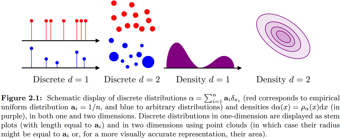
In the figure below, red dots are uniform distributions (\(\mathbf{a}_i = 1/n\)) and blue dots are arbitrary ones. In 1-D, a discrete distribution is drawn as stems (length = weight); in 2-D, as a point cloud (dot size = weight).

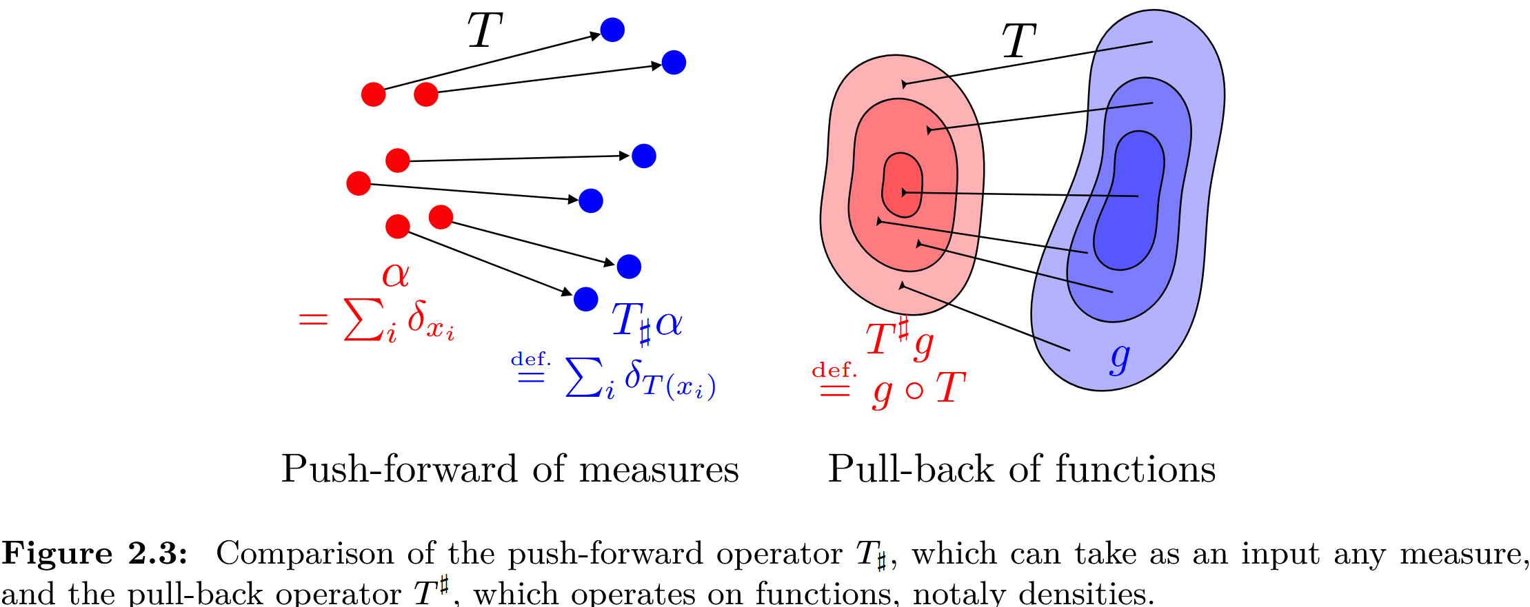
Push-forward operator: for a continuous map \(T:\mathcal{X}\to\mathcal{Y}\), the push-forward operator is \(T_\sharp:\mathcal{M}(\mathcal{X})\to\mathcal{M}(\mathcal{Y})\). For a discrete measure, it simply moves every point to its image under \(T\):

Intuitively, a measurable map \(T\) moves a point in one space to a point in another, and \(T_\sharp\) extends this from single points to whole probability measures: it “pushes” one measure forward into a new one.

2.2 The Monge problem

2.2.1 Definition

The Monge problem: find a map from one measure to another that minimizes the sum of all \(c(x_i, T(x_i))\), where \(c\) is the transport cost and has to be defined for the application at hand.

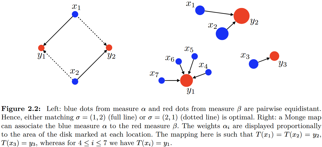
In the discrete setting, given two discrete measures

we look for a map \(T:\{x_1,\ldots,x_n\}\to\{y_1,\ldots,y_m\}\) such that

This constraint can be written compactly as \(T_{\sharp} \alpha=\beta\) and is called the mass conservation constraint.

• When \(n=m\) and the weights are uniform, \(T\) is a one-to-one matching (left figure below);
• When \(n>m\), each \(x_i\) must be sent as a whole to a single \(y_j\), but a \(y_j\) can receive several \(x_i\) (right figure);
• When \(n<m\) (and all \(\mathbf{b}_j > 0\)), at most \(n\) of the \(y_j\) can receive any mass, so the constraint cannot be met and the problem has no solution.

Putting it together, the problem is

In words: through the map \(T\), every \(\mathbf{a}_i\) must be shipped, and each \(\mathbf{b}_j\) must receive exactly its own amount. \(c\) is the transport cost and \(T\) is the transport plan.

2.2.2 Limitations

1. A feasible solution may not exist: e.g. the \(n<m\) case above.
2. The feasible set is non-convex and hard to optimize: the push-forward in the mass conservation constraint is combinatorial, so optimization is hard and often comes down to enumerating plans, which is extremely expensive.

So can we drop the requirement that transport be a deterministic map, and turn OT into a convex problem? Then:

1. a feasible solution always exists (e.g. \(\mathbf{a}\mathbf{b}^{\mathrm{T}}\));
2. we can use a wide range of optimization methods to solve it.

This is the Kantorovich relaxation.

2.3 The Kantorovich relaxation

2.3.1 The transport polytope

Kantorovich’s key idea is to relax the deterministic nature of transport. In the Monge problem, a source point \(x_i\) must be assigned as a whole to a single location \(T(x_i)\); Kantorovich instead allows the mass at \(x_i\) to be split and sent to several targets. In other words, deterministic transport is replaced by probabilistic transport.

For probability vectors \(\mathbf{a}\in\Sigma_n\) and \(\mathbf{b}\in\Sigma_m\), the set of admissible transport plans (couplings) is

where

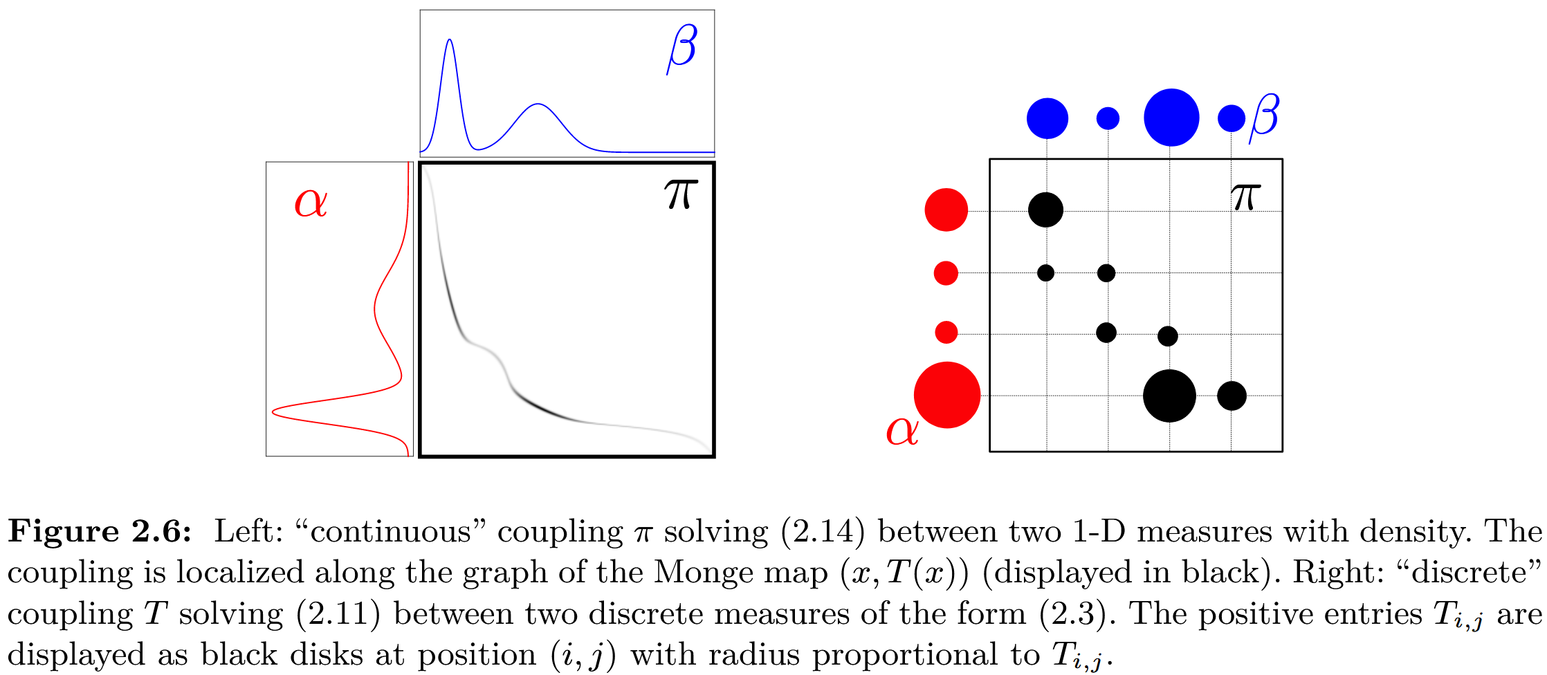
That is, the rows of \(\mathbf{P}\) sum to \(\mathbf{a}\) and its columns sum to \(\mathbf{b}\). The right side of the figure below draws a discrete coupling as a matrix, with disk size proportional to \(\mathbf{P}_{i,j}\):

\(\mathbf{U}(\mathbf{a},\mathbf{b})\) is defined by \(n+m\) linear equality constraints plus non-negativity, so it is a bounded convex polytope (the convex hull of finitely many matrices).

Also, the Monge problem is inherently asymmetric (see the right Monge example above: \(x_4,\ldots,x_7\) can merge into \(y_1\), but \(y_1\) cannot be split back into them), whereas the Kantorovich relaxation is always symmetric: \(\mathbf{P}\in\mathbf{U}(\mathbf{a},\mathbf{b})\) if and only if \(\mathbf{P}^{\mathrm{T}}\in\mathbf{U}(\mathbf{b},\mathbf{a})\).

2.3.2 The objective and how to read it

The resulting optimization problem is

Some ways to read it:

1. The inner product of \(\mathbf{C}\) and \(\mathbf{P}\) should be as small as possible, i.e. pairs of points with lower transport cost get larger matching weights \(\mathbf{P}_{i,j}\);
2. Kantorovich relaxes the constraint, allowing many-to-many matching between \(x\) and \(y\);
3. The rows of \(\mathbf{P}^*\) sum to \(\mathbf{a}\) and its columns to \(\mathbf{b}\), i.e. total input and output must match;
4. Since the row and column sums of \(\mathbf{P}^*\) are both probability distributions, \(\mathbf{P}^*\) can also be read as a joint probability distribution.

2.3.3 Monge vs. Kantorovich

• Motivation: Kantorovich relaxes Monge’s mass conservation constraint by introducing mass splitting: the mass at a source point \(x_i\) can be spread across different destinations;
• Idea: from deterministic transport to probabilistic transport;
• Solving: the Monge problem is non-convex and may have no feasible solution; the Kantorovich problem is a linear program, always has an optimal solution, and can be solved with mature LP methods;
• Generality: the Kantorovich formulation greatly broadens where OT can be applied.

3. Algorithms

3.1 Exact solutions

Solving OT usually means solving the Kantorovich relaxation, which is a linear program.

3.1.1 Vertices of the transport polytope

A linear program with a non-empty, bounded feasible set always attains its minimum at some vertex of that set. Since \(\mathbf{U}(\mathbf{a},\mathbf{b})\) is bounded, the search for an optimal \(\mathbf{P}\) can be restricted to the vertices (extreme points) of \(\mathbf{U}(\mathbf{a},\mathbf{b})\).

3.1.2 A bipartite-graph view

OT can be viewed as a network flow problem on a bipartite graph: \(n\) source nodes on the left, \(m\) target nodes on the right, each edge \((i, j')\) has cost \(\mathbf{C}_{i,j}\), and \(\mathbf{P}_{i,j}\) is the flow on that edge.

A key result: \(\mathbf{P}\) is a vertex of \(\mathbf{U}(\mathbf{a},\mathbf{b})\) if and only if its edges with non-zero flow contain no cycle. This also means a vertex solution has at most \(n+m-1\) non-zero flows.

Each line on the right is a flow of mass. It contains the cycle \((1,1'),(2,1'),(2,4'),(1,4')\), so it is not a vertex. This is the geometric picture behind solving OT.

3.1.3 North-west corner rule and network simplex

• North-west corner rule: start from the top-left entry of the matrix. At each step, put the smaller of “what is left of \(\mathbf{a}_i\)” and “what is left of \(\mathbf{b}_j\)” into the current cell, then move down or right depending on which one ran out. After at most \(n+m-1\) steps this gives a vertex solution: feasible, but usually not optimal.
• Network simplex: start from the north-west corner solution. At each step, add an edge that lowers the total cost and shift flow along the cycle it creates, moving between adjacent vertices until no better neighbor exists.

For \(n\) points, exact solvers cost roughly \(O(n^3\log n)\), which gets slow quickly as the data grows. This is the motivation for entropic regularization.

3.2 Entropic regularization

In most applications, the exact solution of the Kantorovich problem is not needed: solving a regularized version approximately makes OT far cheaper. The entropy is defined as

\(\mathbf{H}\) is 1-strongly concave, since \(\partial^2 \mathbf{H}(\mathbf{P})=-\operatorname{diag}\left(1 / \mathbf{P}_{i, j}\right)\) and \(\mathbf{P}_{i, j} \leq 1\). Entropic regularization uses \(-\mathbf{H}\) as the regularizer and solves for an approximate solution:

The figure below shows the effect of \(\varepsilon\): at \(\varepsilon = 0\) the solution sits on a vertex of the feasible set (the LP solution); as \(\varepsilon\) grows, the entropy pushes the solution away from the boundary toward the “entropic center” inside the feasible set.

Seen on the coupling matrix, entropic regularization penalizes sparse plans made of a few high-flow paths and favors spreading the mass over many low-flow paths. The larger \(\varepsilon\), the blurrier and more spread out the coupling (it tends to \(\mathbf{a}\mathbf{b}^{\mathrm{T}}\) as \(\varepsilon\to\infty\)); the smaller \(\varepsilon\), the closer it gets to the sparse exact solution.

With the entropy term, the objective becomes strongly convex and the optimal solution has a very simple structure, which the Sinkhorn iterations in the next section exploit. That is why entropic regularization cuts the cost so much.

Aside: quadratic regularization. Besides entropy, one can also regularize with the quadratic term \(\|\mathbf{P}\|^2\). Its main advantage over entropy is that the optimal coupling is a sparse approximation, but the solvers are slower and cannot be parallelized as efficiently as Sinkhorn to compute many OT problems at once. In the figure below, the top row is entropic and the bottom row is quadratic:

3.3 The Sinkhorn algorithm

Sinkhorn is exactly the algorithm for the entropic problem above: one can show that the optimal solution always has the form \(\operatorname{diag}(u)\,K\,\operatorname{diag}(v)\), so all we need is to alternately rescale two vectors \(u\) and \(v\) until the row and column sums match the two marginals. Once we have \(u\) and \(v\), we have the optimal coupling of the regularized problem, which approximates the original one. Below we follow Cuturi (2013) through the derivation.

3.3.1 Notation

\(r\) and \(c\) are two probability vectors in the simplex \(\Sigma_d:=\{x\in \mathbb{R}_{+}^{d}: x^{\mathrm{T}}\mathbf{1}_d=1\}\). The transport polytope is

\(P\) can be read as a joint distribution whose marginals are \(r\) and \(c\). \(M\) is the cost matrix; the paper takes it to be a distance matrix (zero on the diagonal and satisfying the triangle inequality):

The objective is

3.3.2 Sinkhorn distances

The idea is the same as before: to make the solution less sparse, increase its entropy. The coupling with the largest entropy in \(U(r,c)\) is the independent coupling \(rc^{\mathrm{T}}\): every entry is \(r_i c_j\), all strictly positive as long as \(r\) and \(c\) are, so it is the “densest” possible plan.

So we add a constraint that keeps \(P\) from straying too far from \(rc^{\mathrm{T}}\):

and define the Sinkhorn distance

As the figure shows, the Sinkhorn distance is the inner product of \(M\) with the optimal transport plan inside this KL ball.

A classic inequality from information theory (Cover & Thomas, 1991) says that the joint entropy never exceeds the sum of the marginal entropies:

Expanding the KL divergence then gives

We now prove the identity used here:

The KL divergence, entropy, and cross-entropy are defined as

and \(\mathrm{KL}(P\|Q)=H(P,Q)-h(P)\). So it suffices to show that \(H(P,rc^{\mathrm{T}})=h(r)+h(c)\):

The third step uses that the rows of \(P\) sum to \(r\) and its columns to \(c\). ∎

Back to the constraint \(h(P) \geq h(r)+h(c)-\alpha\): \(h(r)\) and \(h(c)\) are constants, so the constraint just says that \(h(P)\) is at least some constant. By Lagrangian duality, for every \(\alpha\) there is a \(\lambda>0\) such that the constrained problem is equivalent to minimizing

i.e. we want \(h(P)\) to be as large as possible. This is the same problem as the entropic regularization in Section 3.2 (with \(\lambda = 1/\varepsilon\); the two entropies differ only by a constant).

Adding the marginal constraints, the Lagrangian is

Setting the partial derivative with respect to \(p_{ij}\) to zero:

Let \(u_{i}=e^{-\frac{1}{2}-\lambda \alpha_{i}}\), \(v_{j}=e^{-\frac{1}{2}-\lambda \beta_{j}}\), and \(K_{ij}=e^{-\lambda m_{ij}}\). In matrix form this is

So the only unknowns are \(u\) and \(v\). Plugging into the marginal constraints:

This gives the update rules for \(u\) and \(v\), applied alternately as a fixed-point iteration until convergence:

Each step is just a matrix–vector product plus an element-wise division, which makes it well suited to batched computation on GPUs, and the iteration can be shown to converge linearly.

4. OT in practice

4.1 Wasserstein GAN (ICML 2017)

Replaces the JS divergence in the original GAN objective with the Wasserstein-1 distance (via Kantorovich–Rubinstein duality). When the supports of the two distributions barely overlap, the JS divergence gives vanishing gradients, while the Wasserstein distance still provides meaningful ones, so training is more stable.

4.2 Missing-data imputation with OT (ICML 2020)

Combines the Wasserstein distance, entropic regularization, and the Sinkhorn algorithm. The core idea: two batches drawn at random from the same dataset should come from the same distribution, so the Sinkhorn divergence between them should be small. Treating the missing values as optimization variables and minimizing the Sinkhorn divergence between batches gives the imputed values.

4.3 Neural Optimal Transport (ICLR 2023 Spotlight)

Learns a stochastic OT map \(T(x, z)\) with neural networks: the same input \(x\) combined with different noise \(z\) can map to multiple samples of the target distribution. This enables both one-to-one and one-to-many transfer, with a parameter that controls the diversity of the outputs. Code: iamalexkorotin/NeuralOptimalTransport.

References

1. G. Peyré, M. Cuturi. Computational Optimal Transport. Foundations and Trends in Machine Learning, 2019.
2. M. Cuturi. Sinkhorn Distances: Lightspeed Computation of Optimal Transport. NeurIPS, 2013.
3. T. M. Cover, J. A. Thomas. Elements of Information Theory. Wiley, 1991.
4. M. Arjovsky, S. Chintala, L. Bottou. Wasserstein Generative Adversarial Networks. ICML, 2017.
5. B. Muzellec, J. Josse, C. Boyer, M. Cuturi. Missing Data Imputation using Optimal Transport. ICML, 2020.
6. A. Korotin, D. Selikhanovych, E. Burnaev. Neural Optimal Transport. ICLR, 2023.

1. 最优运输问题简述

给定一个源分布和一个目标分布，我们希望用最小的总代价把源分布”搬运”成目标分布。其中 \(c(m,n)\) 是把单位质量从 \(m\) 运到 \(n\) 的代价，要求的是最优的运输方案 \(p(m,n)\)。

求出最小总代价和最优运输方案之后，我们就可以：

• 用最小总代价来衡量两个分布之间的相似性或差异性；
• 在一定条件下，用运输方案 \(p(m,n)\) 对新的样本做类似的迁移。

2. 概念引入

2.1 基础概念

Histograms（概率向量 / 概率直方图）：一个长度为 \(n\) 的数组，每个元素都在 \([0, 1]\) 之间，且总和为 1，即表示一个离散的概率分布：

Discrete measures（离散测度）：一个带有权重 \(\mathbf{a}\)、位置为 \(x_1, \ldots, x_n \in \mathcal{X}\) 的离散测度写作

下图中红色点是均匀分布（\(\mathbf{a}_i = 1/n\)），蓝色点是任意分布。一维的离散分布画成竖线（长度即权重），二维的离散分布画成点云（点的大小表示权重）。

Push-forward operator（前推算子）：对于连续映射 \(T:\mathcal{X}\to\mathcal{Y}\)，定义前推算子 \(T_\sharp:\mathcal{M}(\mathcal{X})\to\mathcal{M}(\mathcal{Y})\)。对于离散测度，前推算子就是把测度中每个点的位置都用 \(T\) 移动一下：

直观地说，可测映射 \(T\) 把一个空间中的点移动到另一个空间中的点，而 \(T_\sharp\) 是它的扩展：作用对象从单个点变成了整个概率测度，把一个测度整体”推”成一个新的测度。

2.2 蒙日（Monge）问题

2.2.1 定义

Monge 问题：找一个从一个测度到另一个测度的映射，使得所有 \(c(x_i, T(x_i))\) 的和最小。其中 \(c\) 表示运输代价，需要根据具体应用来定义。

用离散测度来说，对于两个离散测度

我们要找一个映射 \(T:\{x_1,\ldots,x_n\}\to\{y_1,\ldots,y_m\}\)，使得

这个约束可以简写为 \(T_{\sharp} \alpha=\beta\)，称为质量守恒约束（mass conservation constraint）。

• \(n=m\) 且权重均匀时，\(T\) 就是一个一一对应的匹配，如下左图；
• \(n>m\) 时，一个 \(x_i\) 只能整体送到一个 \(y_j\)，但一个 \(y_j\) 可以接收多个 \(x_i\)，如下右图；
• \(n<m\) 时（且 \(\mathbf{b}_j\) 都大于 0），最多只有 \(n\) 个 \(y_j\) 能收到质量，约束无法满足，问题无解。

最终的形式化表达为

含义是：通过映射 \(T\)，所有 \(\mathbf{a}_i\) 都必须被运走，并且每个 \(\mathbf{b}_j\) 收到的总量恰好等于它自己。其中 \(c\) 代表运输代价，\(T\) 就是运输方案。

2.2.2 缺陷

1. 不一定存在可行解：例如上面说的 \(n<m\) 的情况。
2. 可行域非凸，求解效率低：质量守恒约束里的 push-forward 是一个组合约束，使得优化非常困难，很多时候只能枚举方案，复杂度极高。

那么能否去掉 push-forward 这种”确定性映射”的约束，把整个 OT 问题变成凸问题？这样一来：

1. 可行解总是存在（例如 \(\mathbf{a}\mathbf{b}^{\mathrm{T}}\)）；
2. 可以灵活地使用各种优化方法求解。

这就是 Kantorovich 松弛。

2.3 Kantorovich 松弛

2.3.1 运输多面体

Kantorovich 的关键想法是放宽运输的”确定性”：在 Monge 问题里，源点 \(x_i\) 只能整体分配给一个位置 \(T(x_i)\)；而 Kantorovich 允许 \(x_i\) 的质量被拆分，分别送往多个目标点。也就是说，他放弃了确定性运输，转而考虑概率运输（probabilistic transport）。

对于概率向量 \(\mathbf{a}\in\Sigma_n\) 和 \(\mathbf{b}\in\Sigma_m\)，可行的运输方案（耦合）集合定义为

其中

即 \(\mathbf{P}\) 的行和等于 \(\mathbf{a}\)，列和等于 \(\mathbf{b}\)。下图右侧把一个离散耦合画成矩阵，黑点的大小表示 \(\mathbf{P}_{i,j}\)：

\(\mathbf{U}(\mathbf{a},\mathbf{b})\) 由 \(n+m\) 个线性等式约束加上非负约束定义，是一个有界的凸多面体（有限个矩阵的凸包）。

此外，Monge 问题本质上是不对称的（见上面 Monge 例子的右图：\(x\) 可以合并到 \(y\)，但反过来 \(y_1\) 无法拆回 \(x_4,\ldots,x_7\)），而 Kantorovich 松弛总是对称的：\(\mathbf{P}\in\mathbf{U}(\mathbf{a},\mathbf{b})\) 当且仅当 \(\mathbf{P}^{\mathrm{T}}\in\mathbf{U}(\mathbf{b},\mathbf{a})\)。

2.3.2 求解公式与理解

最终的优化问题为

对这个式子的理解：

1. \(\mathbf{C}\) 与 \(\mathbf{P}\) 的矩阵内积要尽可能小，即运输代价越小的两个点，获得越大的匹配权重 \(\mathbf{P}_{i,j}\)；
2. Kantorovich 松弛了约束，允许多个 \(x\) 到多个 \(y\) 的匹配；
3. \(\mathbf{P}^*\) 的行和等于 \(\mathbf{a}\)，列和等于 \(\mathbf{b}\)，即输入与输出的总量要匹配；
4. 因为 \(\mathbf{P}^*\) 的行和、列和分别是两个概率分布，\(\mathbf{P}^*\) 也可以理解为一个联合概率分布矩阵。

2.3.3 对比 Monge 与 Kantorovich

• 动机：Kantorovich 松弛了 Monge 问题的质量守恒约束，引入 mass splitting，即源点 \(x_i\) 的质量可以分散地运到不同地方；
• 思想：从确定性运输（deterministic transport）变成概率运输（probabilistic transport）；
• 求解：Monge 问题非凸，且不一定有可行解；Kantorovich 问题是一个线性规划，一定存在最优解，并且可以用成熟的线性规划方法求解；
• 泛化性：Kantorovich 形式极大地扩展了 OT 的应用场景。

3. 算法求解

3.1 精确求解

最优运输问题的求解一般指求 Kantorovich 松弛的解，它是一个线性规划。

3.1.1 运输多面体的顶点

可行集非空且有界的线性规划，一定能在可行集的某个顶点处取到最小值。由于 \(\mathbf{U}(\mathbf{a},\mathbf{b})\) 是有界的，可以把最优 \(\mathbf{P}\) 的搜索范围限制在多面体 \(\mathbf{U}(\mathbf{a},\mathbf{b})\) 的顶点（极值点）上。

3.1.2 二分图视角

可以把 OT 看成二分图上的网络流问题：左边是 \(n\) 个源点，右边是 \(m\) 个目标点，每条边 \((i, j')\) 的代价为 \(\mathbf{C}_{i,j}\)，\(\mathbf{P}_{i,j}\) 就是这条边上的流量。

一个重要结论是：\(\mathbf{P}\) 是 \(\mathbf{U}(\mathbf{a},\mathbf{b})\) 的顶点，当且仅当它的非零流量边不构成环。这也意味着顶点解中最多只有 \(n+m-1\) 条非零流量。

上图右侧的每条连线表示一条质量流，其中存在环 \((1,1'),(2,1'),(2,4'),(1,4')\)，所以它不是一个顶点。这就是最优运输问题的几何解释。

3.1.3 西北角法与网络单纯形法

• 西北角法（North-west corner rule）：从矩阵左上角开始，每次在当前位置放入”剩余的 \(\mathbf{a}_i\)“和”剩余的 \(\mathbf{b}_j\)“中较小的那个，哪边先用完就向下或向右移动一格。最多 \(n+m-1\) 步就能得到一个顶点解，它是可行的，但通常不是最优的。
• 网络单纯形法（Network simplex）：以西北角法的结果为初始解，每次加入一条能降低总代价的边，并沿着产生的环调整流量，在相邻顶点之间移动，直到找不到更优的顶点为止。

精确求解在 \(n\) 个点时的复杂度大约是 \(O(n^3\log n)\) 量级，数据量一大就很慢，这也是后面要引入熵正则化的原因。

3.2 熵（Entropic）正则化

在大部分应用中，求出 Kantorovich 问题的精确解是不必要的：如果改用正则化求近似解，最优运输的计算代价会大幅降低。熵的定义为

\(\mathbf{H}\) 是 1-强凹（strongly concave）的，因为 \(\partial^2 \mathbf{H}(\mathbf{P})=-\operatorname{diag}\left(1 / \mathbf{P}_{i, j}\right)\) 且 \(\mathbf{P}_{i, j} \leq 1\)。熵正则化就是用 \(-\mathbf{H}\) 作为正则项，求一个近似解：

下图展示了 \(\varepsilon\) 的影响：\(\varepsilon = 0\) 时解落在可行域的顶点上（即 LP 的解）；随着 \(\varepsilon\) 增大，熵把解逐渐推离边界，移向可行域内部的”熵中心”。

从耦合矩阵上看，熵正则化惩罚由少数几条大流量路径组成的稀疏方案，鼓励把质量分散到许多小流量路径上。\(\varepsilon\) 越大，耦合越模糊、越分散（\(\varepsilon\to\infty\) 时趋向 \(\mathbf{a}\mathbf{b}^{\mathrm{T}}\)）；\(\varepsilon\) 越小，越接近稀疏的精确解。

加了熵之后，目标函数变成强凸的，最优解有非常简单的结构，可以用下一节的 Sinkhorn 迭代快速求解，这就是熵正则化能大幅降低计算代价的原因。

补充：二次正则化。 除了熵，也可以用二次项 \(\|\mathbf{P}\|^2\) 做正则。和熵相比，它的主要优点是得到的最优耦合是稀疏的近似，但代价是求解更慢，也不能像 Sinkhorn 那样高效地并行、同时计算多个最优运输问题。下图上面一行是熵正则化，下面一行是二次正则化：

3.3 Sinkhorn 算法

Sinkhorn 算法正是求解上面熵正则化问题的方法：可以证明最优解一定具有 \(\operatorname{diag}(u)\,K\,\operatorname{diag}(v)\) 的形式，只需要交替缩放两个向量 \(u\) 和 \(v\)，让行和、列和分别等于两个边缘分布即可。得到 \(u\) 和 \(v\)，就得到了正则化问题的最优耦合，它是原问题的一个近似解。下面沿着 Cuturi (2013) 的思路推导一遍。

3.3.1 符号整理

\(r\) 与 \(c\) 是两个概率向量，属于单纯形 \(\Sigma_d:=\{x\in \mathbb{R}_{+}^{d}: x^{\mathrm{T}}\mathbf{1}_d=1\}\)。运输多面体（transport polytope）为

\(P\) 可以理解为联合概率分布，它的两个边缘分布分别是 \(r\) 与 \(c\)。\(M\) 是代价矩阵，原文取为一个距离矩阵（对角线为 0，且满足三角不等式）：

优化目标为

3.3.2 Sinkhorn distances

思路仍然是：想让解不那么稀疏，就要让它的熵更大。在 \(U(r,c)\) 中熵最大的是独立耦合 \(rc^{\mathrm{T}}\)：它的每个元素是 \(r_i c_j\)，只要 \(r\)、\(c\) 严格为正就全都大于 0，是最”稠密”的运输方案。

于是加上约束，让 \(P\) 不能离 \(rc^{\mathrm{T}}\) 太远：

并定义 Sinkhorn 距离

如下图所示，Sinkhorn 距离就是 \(M\) 与这个 KL 球中最优运输方案的内积。

由信息论中的经典不等式（Cover & Thomas, 1991），联合熵不超过边缘熵之和：

再把 KL 散度展开，可以得到

下面证明其中用到的等式

KL 散度、熵和交叉熵的定义分别为

并且 \(\mathrm{KL}(P\|Q)=H(P,Q)-h(P)\)。所以只需证明 \(H(P,rc^{\mathrm{T}})=h(r)+h(c)\)：

第三步用到了 \(P\) 的行和为 \(r\)、列和为 \(c\)。证毕。

回到约束 \(h(P) \geq h(r)+h(c)-\alpha\)：其中 \(h(r)\) 与 \(h(c)\) 都是常数，所以约束就是 \(h(P)\) 不小于某个常数。根据拉格朗日对偶，对每个 \(\alpha\) 都存在一个 \(\lambda>0\)，使得这个带约束的问题等价于最小化

也就是希望 \(h(P)\) 尽可能大。它和 3.2 节的熵正则化是同一个问题（\(\lambda = 1/\varepsilon\)，两者的熵只差一个常数）。

再把边缘分布的约束加上，写出拉格朗日函数：

对 \(p_{ij}\) 求偏导并令其为 0：

记 \(u_{i}=e^{-\frac{1}{2}-\lambda \alpha_{i}}\)，\(v_{j}=e^{-\frac{1}{2}-\lambda \beta_{j}}\)，\(K_{ij}=e^{-\lambda m_{ij}}\)，写成矩阵形式就是

所以我们真正要解的只有 \(u\) 和 \(v\)。代入边缘分布的约束：

由此得到 \(u\)、\(v\) 的迭代公式，用不动点迭代交替更新，直到收敛：

每一步只是一次矩阵-向量乘法加逐元素除法，很适合在 GPU 上批量计算，并且可以证明这个迭代是线性收敛的。

4. OT 的实际应用

4.1 Wasserstein GAN（ICML 2017）

用 Wasserstein-1 距离（借助 Kantorovich–Rubinstein 对偶）替代原始 GAN 中的 JS 散度作为训练目标。当两个分布的支撑集几乎不重叠时，JS 散度的梯度会消失，而 Wasserstein 距离依然能给出有意义的梯度，训练更稳定。

4.2 用最优运输做缺失值填补（ICML 2020）

结合了 Wasserstein 距离、熵正则化和 Sinkhorn 算法。核心想法是：从同一个数据集里随机抽出的两个 batch 应该来自同一个分布，所以它们之间的 Sinkhorn 散度应该很小；把缺失值当作优化变量，最小化 batch 之间的 Sinkhorn 散度，就得到了填补结果。

4.3 Neural Optimal Transport（ICLR 2023 Spotlight）

用神经网络学习一个随机的 OT 映射 \(T(x, z)\)：同一个输入 \(x\) 配合不同的噪声 \(z\)，可以映射到目标分布中的多个样本，从而实现一对一和一对多的迁移，并且提供参数来控制生成结果的多样性。代码见 iamalexkorotin/NeuralOptimalTransport。

参考文献

1. G. Peyré, M. Cuturi. Computational Optimal Transport. Foundations and Trends in Machine Learning, 2019.
2. M. Cuturi. Sinkhorn Distances: Lightspeed Computation of Optimal Transport. NeurIPS, 2013.
3. T. M. Cover, J. A. Thomas. Elements of Information Theory. Wiley, 1991.
4. M. Arjovsky, S. Chintala, L. Bottou. Wasserstein Generative Adversarial Networks. ICML, 2017.
5. B. Muzellec, J. Josse, C. Boyer, M. Cuturi. Missing Data Imputation using Optimal Transport. ICML, 2020.
6. A. Korotin, D. Selikhanovych, E. Burnaev. Neural Optimal Transport. ICLR, 2023.